NASA earthaccess and Xarray
Preliminaries
Create Your .netrc File | Earthdata Login Documentation
A simple utility script that will prompt for your Earthdata Login username and password, and create (or update) the .netrc file. Just download and run!
perl create_netrc.pl
OSCAR third degree resolution ocean surface currents - yearly files
Short Name: OSCAR_L4_OC_third-deg_YEARLY

earthaccess
We modify the example Python code for earthaccess:
#Import packages
import earthaccess

#Authentication with Earthdata Login
auth = earthaccess.login(strategy="netrc")

results = earthaccess.search_data(short_name="OSCAR_L4_OC_third-deg_YEARLY",
                                  version="1",
                                  cloud_hosted=True,
                                  temporal = ("2022-01-01","2022-07-31"),
                                  bounding_box = (-51.96423,68.10554,-48.71969,70.70529))

earthaccess.download(results, "./local_folder")
Then local_folder contains the single file, oscar_vel2022.nc.gz. We can use xarray directly with this file. But if we open the file with xarray two or
more times, it becomes quicker to decompress it now. So we run gzip -d oscar_vel2022.nc.gz, and now local_folder contains the single file oscar_vel2022.nc.
Then: 1
import xarray as xr

ds = xr.open_mfdataset("local_folder/oscar_vel2022.nc")
ds.info()
xarray.Dataset {
dimensions:
	time = 72 ;
	year = 72 ;
	depth = 1 ;
	latitude = 481 ;
	longitude = 1201 ;

variables:
	datetime64[ns] time(time) ;
		time:long_name = Day since 1992-10-05 00:00:00 ;
	float32 year(year) ;
		year:units = time in years ;
		year:long_name = Time in fractional year ;
	float32 depth(depth) ;
		depth:units = meter ;
		depth:long_name = Depth ;
	float64 latitude(latitude) ;
		latitude:units = degrees-north ;
		latitude:long_name = Latitude ;
	float64 longitude(longitude) ;
		longitude:units = degrees-east ;
		longitude:long_name = Longitude ;
	float64 u(time, depth, latitude, longitude) ;
		u:units = meter/sec ;
		u:long_name = Ocean Surface Zonal Currents ;
	float64 v(time, depth, latitude, longitude) ;
		v:units = meter/sec ;
		v:long_name = Ocean Surface Meridional Currents ;
	float64 um(time, depth, latitude, longitude) ;
		um:units = meter/sec ;
		um:long_name = Ocean Surface Zonal Currents Maximum Mask ;
	float64 vm(time, depth, latitude, longitude) ;
		vm:units = meter/sec ;
		vm:long_name = Ocean Surface Meridional Currents Maximum Mask ;

// global attributes:
	:VARIABLE = Ocean Surface Currents ;
	:DATATYPE = 1/72 YEAR Interval ;
	:DATASUBTYPE = unfiltered ;
	:GEORANGE = 20 to 420 -80 to 80 ;
	:PERIOD = Jan.01,2022 to Dec.26,2022 ;
	:year = 2022 ;
	:description = OSCAR Third Degree Sea Surface Velocity ;
	:CREATION_DATE = 02:21 06-Feb-2023 ;
	:version = 2009.0 ;
	:source = Gary Lagerloef, ESR ([email protected]) and Kathleen Dohan, ESR ([email protected]) ;
	:contact = Kathleen Dohan ([email protected]) or John T. Gunn ([email protected]) ;
	:company = Earth & Space Research, Seattle, WA ;
	:reference = Bonjean F. and G.S.E. Lagerloef, 2002 ,Diagnostic model and analysis of the surface currents in the tropical Pacific ocean, J. Phys. Oceanogr., 32, 2,938-2,954 ;
	:note1 = Maximum Mask velocity is the geostrophic component at all points + any concurrent Ekman and buoyancy components ;
	:note2 = Longitude extends from 20 E to 420 E to avoid a break in major ocean basins. Data repeats in overlap region. ;
}
Next:
import numpy as np
import cartopy.crs as ccrs
import matplotlib.pyplot as plt

plt.figure(figsize=(18, 9))

ax = plt.axes(projection=ccrs.PlateCarree()) # plate carrée projection

dec = 2

lon = ds.longitude.values[::dec]

lon[lon > 180] = lon[lon > 180] - 360

mymap = plt.streamplot(
    lon,
    ds.latitude.values[::dec],
    ds.u.values[0, 0, ::dec, ::dec],
    ds.v.values[0, 0, ::dec, ::dec],
    8,
    transform = ccrs.PlateCarree()
)

ax.coastlines()

plt.title('Sea surface currents derived from OSCAR')

plt.savefig("currents18x9E.png", dpi=150)

plt.show()
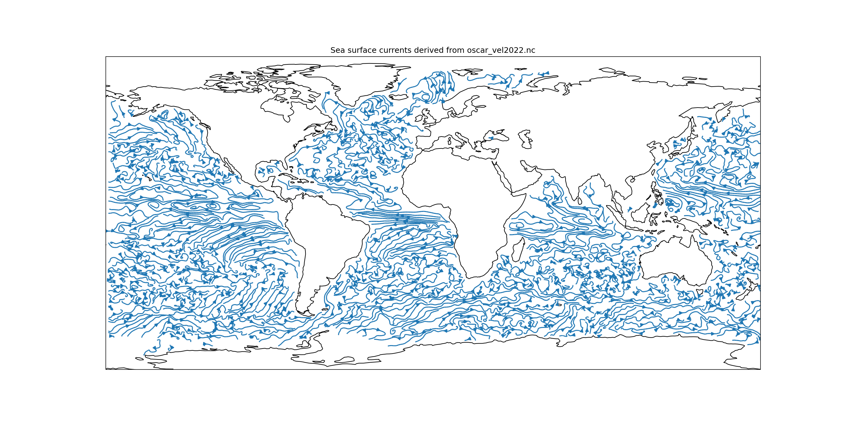
OSCAR 2022 streamplot:

Global sea surface currents, 2022. Streamplot of sea surface velocity from https://t.co/m1l6hzAjiA using Xarray (https://t.co/Pc25mclkus) pic.twitter.com/pcjDKz6uCj
— Jordan Bell (@jordanbell2357) April 29, 2023
My so-far favorite resources for xarray: