Mariquant: Creating sea routes from the sea of AIS data
This post is a gloss on:
Work in progress. When this is ready for any public presentation, I’ll have digested all the original material enough merely to quote a handful of paragraphs and expand on them.
Presently I’ve copied each paragraph of text of the article with space after for my “gloss”, my working through of it, or working out a story of what it means. I do not copy the tables or figures from the article. This is a gloss that expands on the original and the only audience for this post are readers of the original work.
Mariquant has hourly data from one of the AIS data providers for the bulkers and tankers from the beginning of 2016 to the middle of 2018. This data has information from around 19 000 unique ships with records, occupying approximately 100 Gb as uncompressed parquet file.
We have a library of the polygons with approximately 8 000 port harbours and 20 000 anchorage and waiting areas. Most of the time anchorage polygons lay outside of the port polygons, and we used graph algorithms to determine which anchorage belongs to which port. Having this data we started to construct routes.
We will be using the notion of the distance between trajectories to construct the best representation of the route and to separate different trajectories on the same route. Most of the distance calculation algorithms are using the distance between points on the trajectories. We found that some noise prevented us from obtaining meaningful results for the calculations of the distances between trajectories. Looking at the data we found that ships spend a significant amount of time (leading to a large number of points on the trajectories) either anchoring or moving nearby the port harbour.
To find at least some of these points on the trajectories, we used scikit learn[1] implementation of the Random Forest Classifier. There are various approaches to finding different clusters on the vessel trajectories, see for example [2] and references therein. We preferred to use a somewhat simplistic approach as it was easy to implement and provided us with sufficiently accurate results. We used distance to the port, distance to the previous port, speed of the ship, radial velocity of the ship (as if circling the port) and speed in the direction to the port, as the features of the classifier. We manually constructed training and testing sets separately marking ‘loitering’, anchoring, port approaching and general voyage points. We had around 6 400 points in the training and 1600 points in the testing set. Anchoring points are less represented in the sets, as they create fewer problems in the distance calculations. The difficulties in manual markup cause this small size of the set.
The Confusion matrix shows that the loitering, approach and general voyage points are well defined. Even if the approach and general voyage points are misidentified, the misidentification is between two of them, not points of interest.
Precision and recall, together with F1 score show that the results are good, but further improvements may be made for the classifier. We have to repeat that anchoring points are less troublesome for the calculation of the distance between trajectories and we will continue with these results.
We found that distance to the port, distance to the previous port, speed of the ship are the most important features, having a score of 0.42, 0.21 and 0.28 correspondingly and radial speed and speed in the direction to the port have a score of 0.04 and 0.05.
One can use standard Scikit-learn functions to calculate the scores mentioned above.
from sklearn.metrics import classification_report, confusion_matrix
from sklearn.ensemble import RandomForestClassifier
from sklearn.model_selection import train_test_split
X_train, X_test, y_train, y_test = train_test_split(X, y, test_size=0.2, random_state=0)
clf = RandomForestClassifier(n_estimators=20, max_depth=6, random_state=0)
clf.fit(X_train, y_train)
y_pred = clf.predict(X_test)
print(confusion_matrix(y_test, y_pred))
print(classification_report(y_test, y_pred))
print(clf.feature_importances_)
We found that irrespectively from the scores of the classifiers, additional cleanup is required for our large dataset. Sometimes small parts of the port approach trajectories were mistakenly identified as loitering parts, and we had to apply conservative check requiring anchoring and loitering parts of the trajectories to be long enough and either be self-intersecting, or the distance travelled in the direction to the port should be smaller compared to the total length travelled.
After all these checks we average the position of the vessel for the loitering and anchoring parts of the trajectories.
Our approach was inspired by the work of the Philippe Besse, Brendan Guillouet, Jean-Michel Loubes and François Royer [3]. In the original work, authors proposed a new method called ‘Symmetrized segment-path distance’ for distance calculation between trajectories to clusterize taxi voyages to predict final destination point as part of the Kaggle competition [4]. Article [3] has an in-depth description of the various methods for the trajectory distance calculation.
In short, our approach is
- to calculate the distance between trajectories using some measure
- to clusterize trajectories based on their distances.
- to select the “best” trajectory in the cluster.
We tested different methods for the distance calculations and decided to use Edit Distance with Real Penalty (ERP) [5]. This method is a warping distance method and allows comparison between trajectories of different length, aligning trajectories during the computation of the distance between them. It runs in O(n²) time. The implementation of this method is part of the trajectory_distance package created by the authors of [3]. We slightly modified this package to speed-up python part of the calculations and added DASK support for the parallel computations. Due to the memory and calculation time restrictions we select at max 50 random trajectories, as the computation on the popular route may deal with hundreds of them. This leads us to the 43847 distinct routes that will be reconstructed from almost one million trips.
Different trips along the same route can have completely different trajectories. So we need to clusterise these trajectories if needed. Affinity propagation clustering algorithm is the natural choice for this task as it requires neither the initial knowledge of the number of clusters, no triangle inequality for the distance (not all methods for the distance calculations generate distances that satisfy this inequality). We used scikit learn[1] implementation of the Affinity propagation algorithm.
Missing points are usual for the data, collected by the satellites, due to the restrictions of the AIS protocol. We had to find a solution to this problem.
First, we use the cost function that will take into account both the distance between the trajectories (we use simple average) and the number of missing points in the trajectory to define the “best” trajectory.
Second, we update the trajectories iteratively:
We find the “best” trajectory using only available data
We enhance trajectories with the missing points using the “best” trajectory points. Nearest points from the “best” trajectory are found, and the “best” trajectory segment is added to the enhanced trajectory.
We iterate 1 -2 with the additional data until the “best” trajectory remains stable and the value of the cost function diminishes.
After the enhancement of the trajectories, we split trajectories set in the different clusters. “Best” trajectory within each cluster is found using the iterative approach described above. We use these trajectories as the routes between ports.
The data consists of four files:
- Port-to-port distances calculated along the routes (
distances.csv).- Port-to-port routes as discussed above (
routes.csv).- We can’t provide you with the port polygons, however, we provide the reference data consisting of our internal index, World Port Index INDEX_NO, and PORT_NAME if any (or any available name we have) and a tuple of coordinates of the port polygon representative point. Representative point of the harbour polygon is obtained using geopandas representative_point() method (
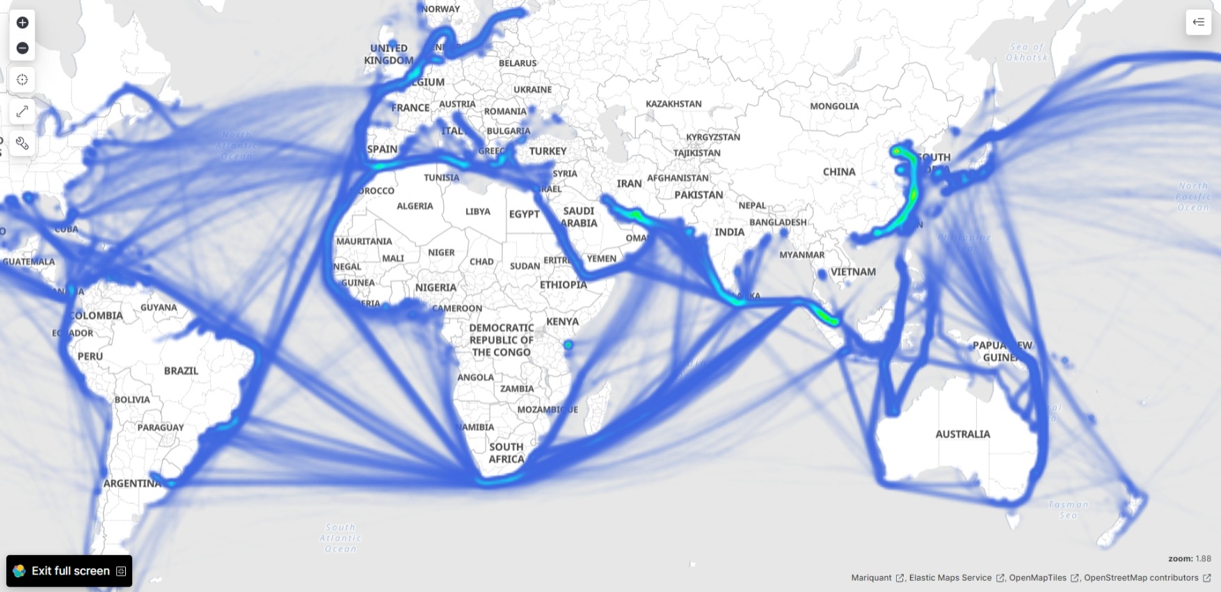
ports.csv).- HTML file with the world map (
WorldRoutes.html)
References
- Pedregosa et al., Scikit-learn: Machine Learning in Python, JMLR 12, pp. 2825–2830, 2011.
- Sheng, Pan, and Jingbo Yin. “Extracting Shipping Route Patterns by Trajectory Clustering Model Based on Automatic Identification System Data.” Sustainability 10.7 (2018): 2327.
- P. Besse, B. Guillouet, J.-M. Loubes, and R. Francois, “Review and perspective for distance based trajectory clustering” arXiv preprint arXiv:1508.04904, 2015.
- ECML/PKDD 15: Taxi Trajectory Prediction (I)
- L. Chen and R. Ng, “On the marriage of lp-norms and edit distance,” Proceedings of the Thirtieth international conference on Very large data bases-Volume 30. VLDB Endowment, 2004, pp. 792–803.
424M    WorldRoutes.html
2.9M    distances.csv
172K    ports.csv
633M    routes.csv
633M    routes_noheader.csv
sklearn.ensemble.RandomForestClassifier
sklearn.cluster.AffinityPropagation
WorldRoutes.html
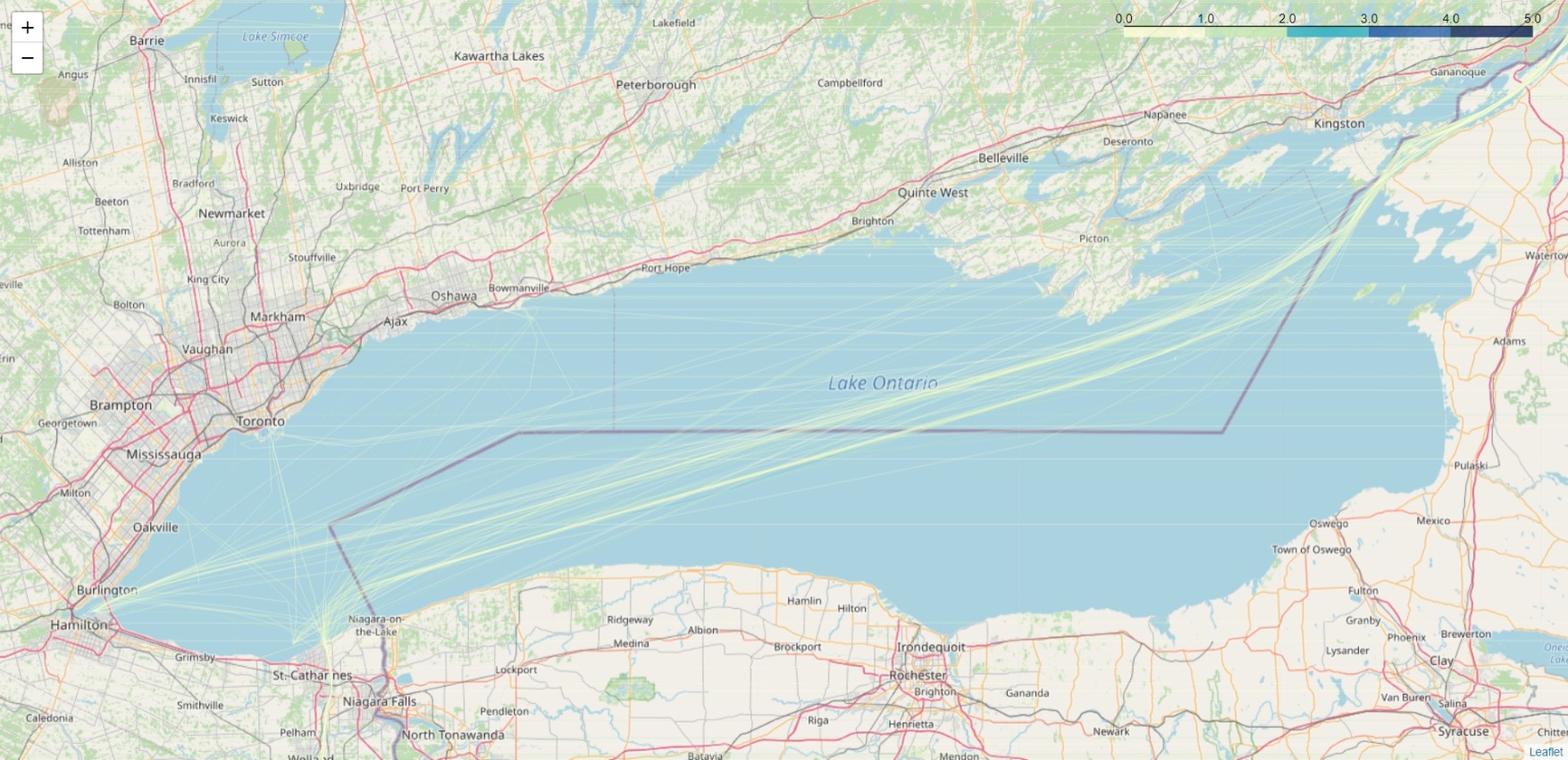
Lake Ontario:
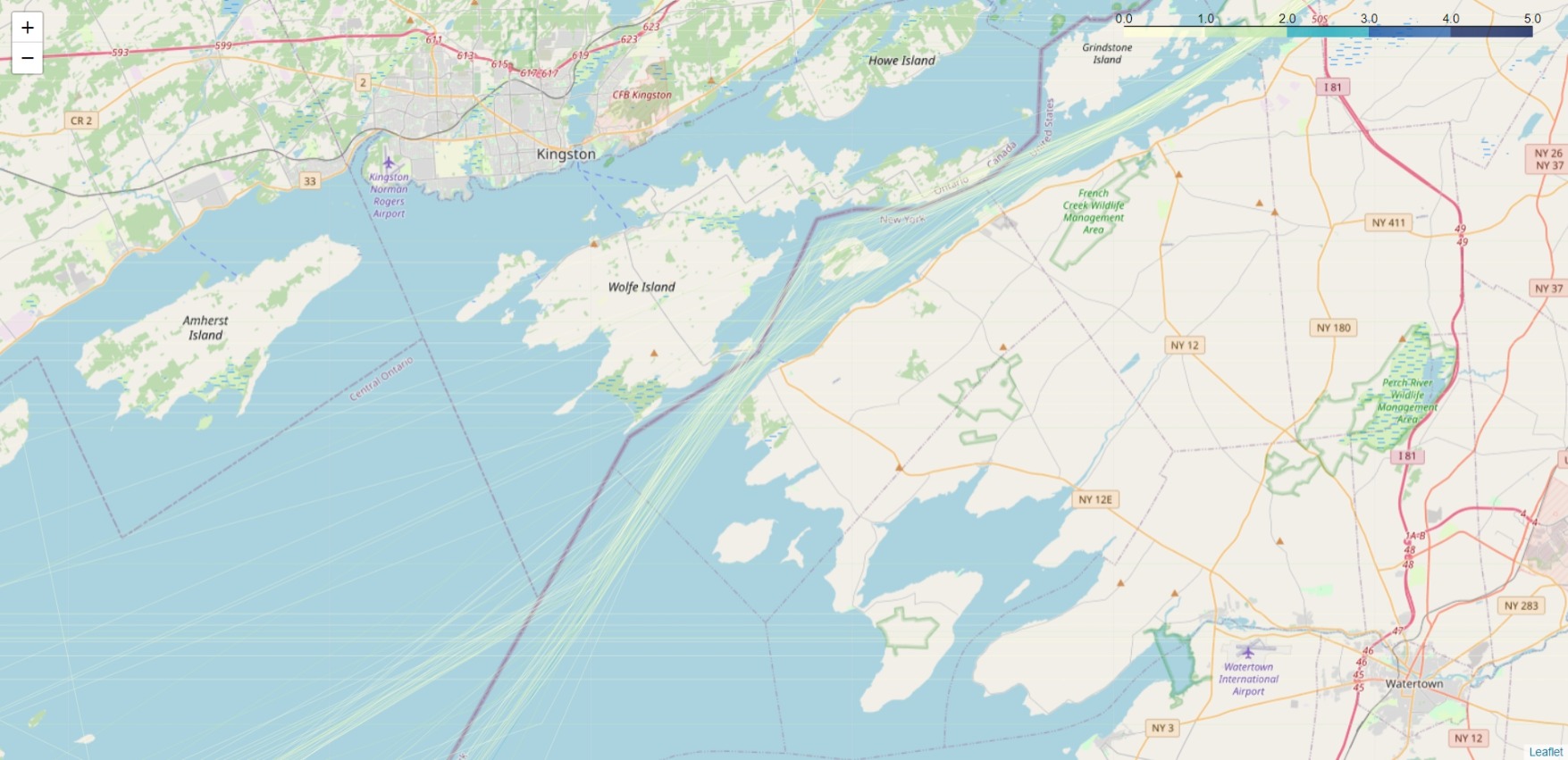
St. Lawrence River:
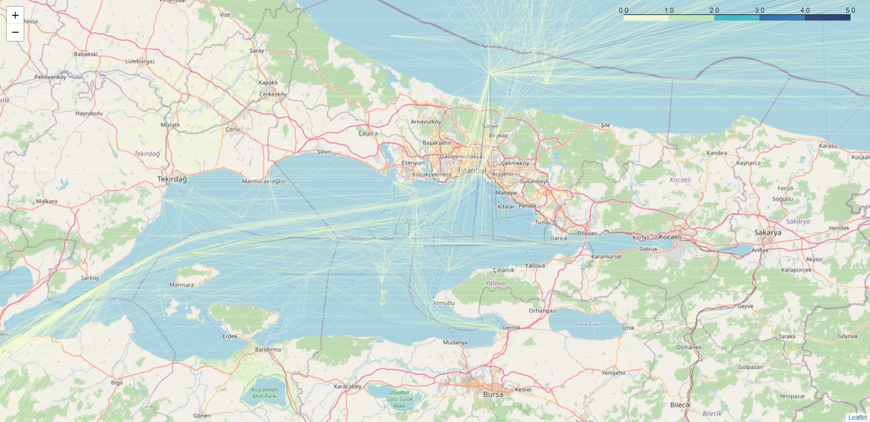
Sea of Marmara:
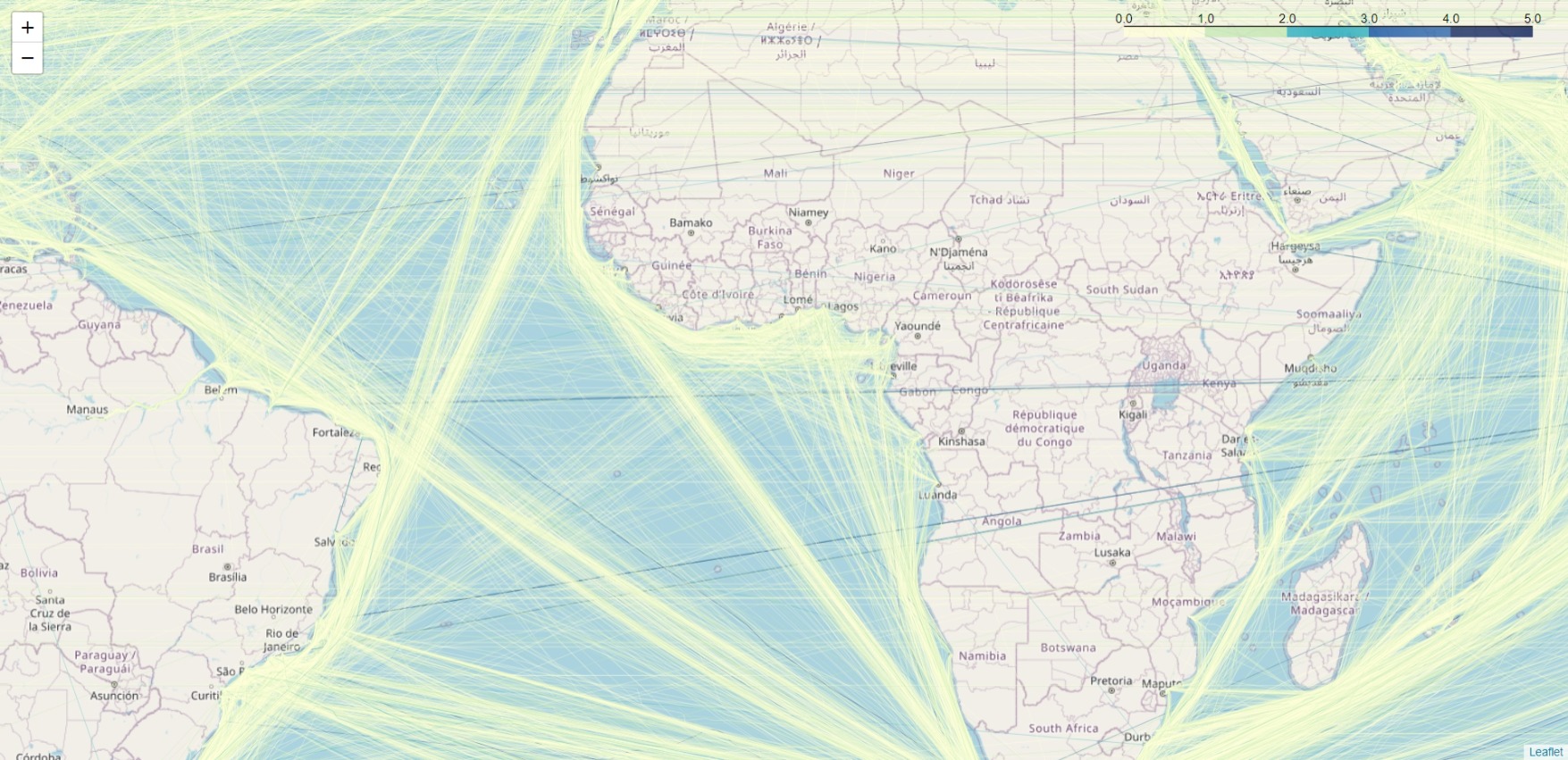
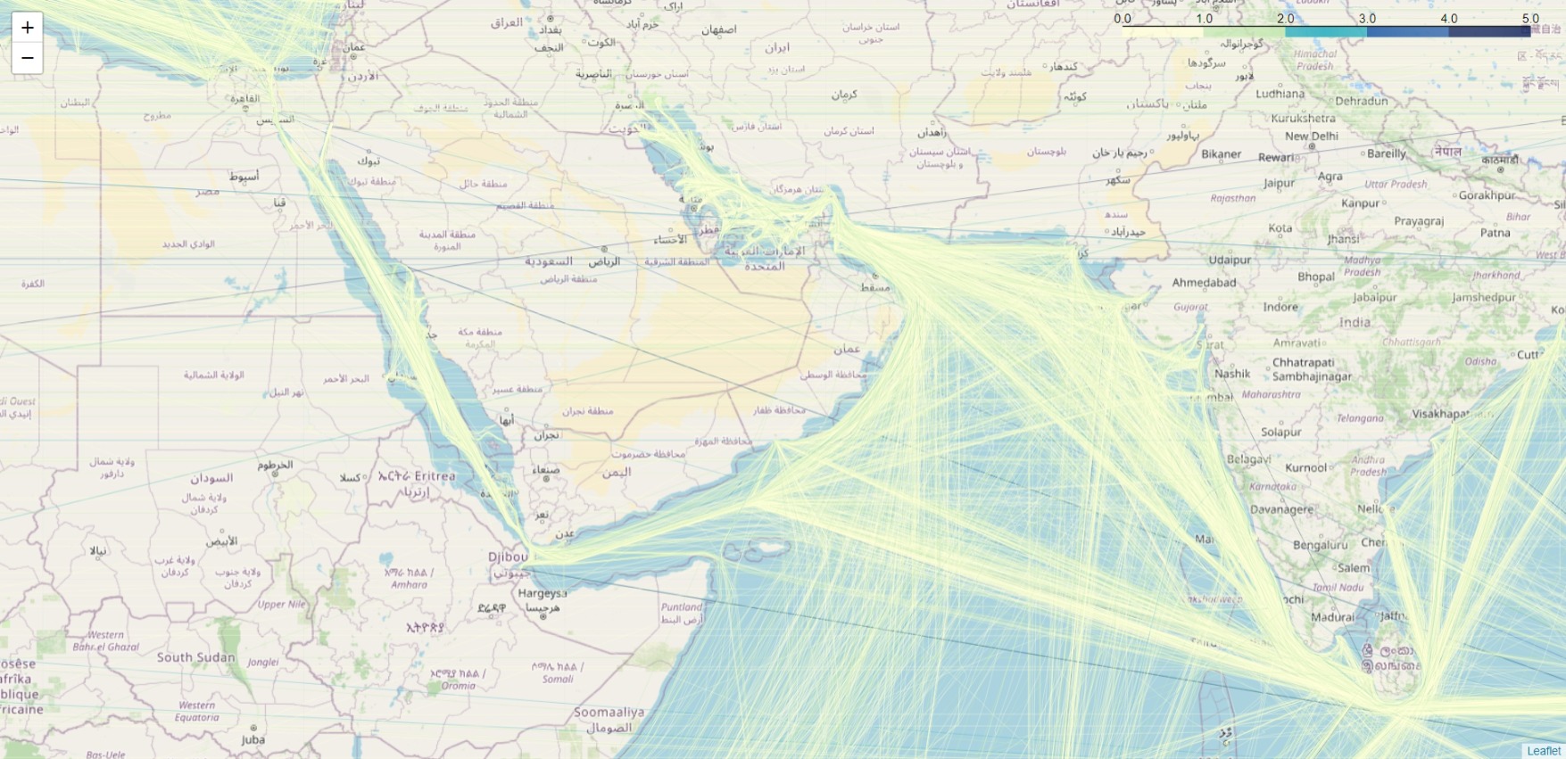
Red Sea and Indian Ocean:
head -n 5 distances.csv
,trip_count,prev_port,next_port,distance,frequency
7682,1984063,4410,3658,460.63814769485793,1.0
7062,1948666,3658,7083,372.7538137212947,1.0
2712,1287366,7083,7084,26.578905957417856,1.0
7248,1950728,7084,2814,9.200891935648707,1.0
head -n 5 ports.csv
,PORT_NAME,INDEX_NO,coords
49159,Terminal Pesquero Cta. Quiane,,"((-70.31722387298942, -18.513597026467323),)"
49164,Oil Berth,,"((-61.86886473007713, 17.150384410999997),)"
16,Port of Basamuk,,"((146.14295817405977, -5.53913255687803),)"
26,Victoria,,"((-123.32715191091728, 48.402783083729446),)"
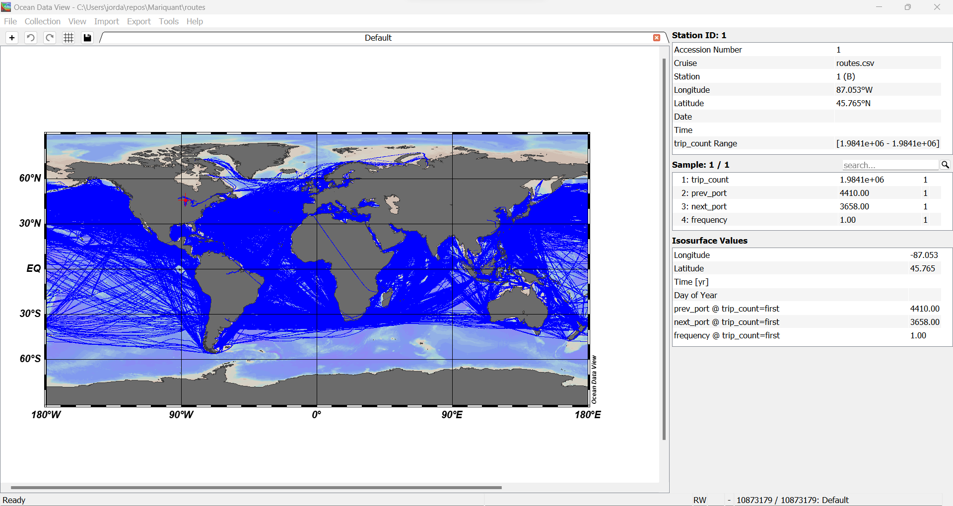
head -n 5 routes.csv
,trip_count,prev_port,next_port,lat,lon,frequency
7641,1984063,4410,3658,45.764835,-87.05328753692308,1.0
7642,1984063,4410,3658,45.60853333,-87.03821667,1.0
7643,1984063,4410,3658,45.56013333,-87.03423333,1.0
7644,1984063,4410,3658,45.48103333,-87.01585,1.0
wc -l routes.csv
10882102 routes.csv
routes.csv using Ocean Data View (ODV):
shuf
sed '1d' routes.csv > routes_noheader.csv
NUMROUTES=1000000
head -n 1 routes.csv > routes_shuf_$NUMROUTES.csv
shuf -n $NUMROUTES routes_noheader.csv >> routes_shuf_$NUMROUTES.csv
59M routes_shuf_1000000.csv
sed
HEADER_ROW=$(head -n 1 routes.csv)
for i  in {1..11}; do echo $HEADER_ROW > routes_to_${i}000000.csv; done
sed -n 2,1000001p routes.csv >> routes_to_1000000.csv
sed -n 1000002,2000001p routes.csv >> routes_to_2000000.csv
sed -n 2000002,3000001p routes.csv >> routes_to_3000000.csv
sed -n 3000002,4000001p routes.csv >> routes_to_4000000.csv
sed -n 4000002,5000001p routes.csv >> routes_to_5000000.csv
sed -n 5000002,6000001p routes.csv >> routes_to_6000000.csv
sed -n 6000002,7000001p routes.csv >> routes_to_7000000.csv
sed -n 7000002,8000001p routes.csv >> routes_to_8000000.csv
sed -n 8000002,9000001p routes.csv >> routes_to_9000000.csv
sed -n 9000002,10000001p routes.csv >> routes_to_10000000.csv
sed -n '10000002,$p' routes.csv >> routes_to_11000000.csv
Elastic Maps Service
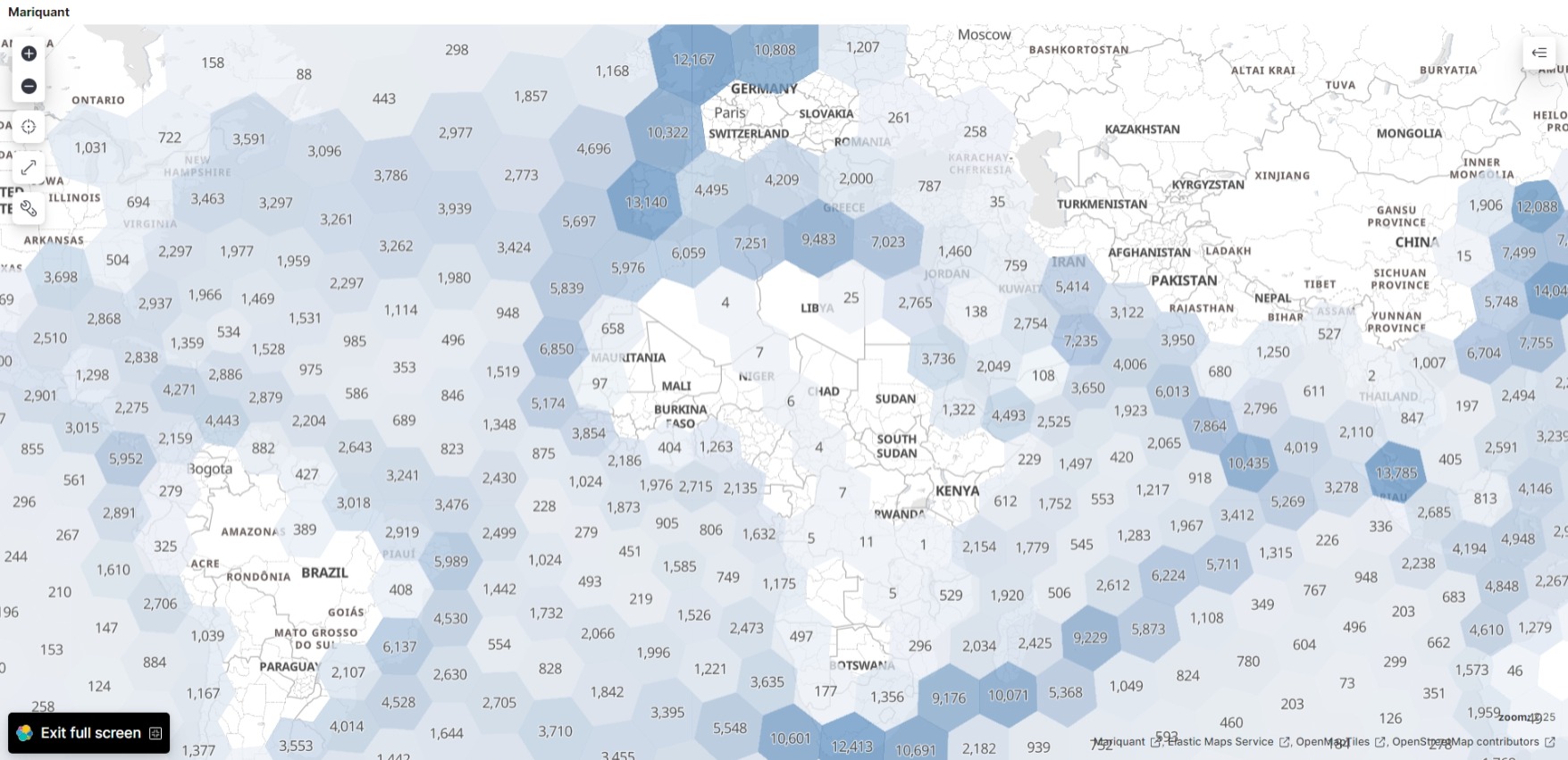
We use Elastic Maps Service first with the random sample routes_shuf_1000000.csv of 1000000 (one million) rows to make hexagon clusters showing vessel count in each hexagon:
Now we visualize the routes_to_${i}000000.csv files using Elastic Maps Service.
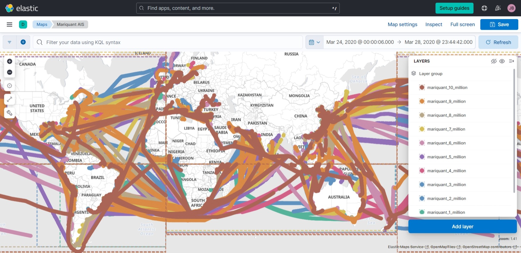
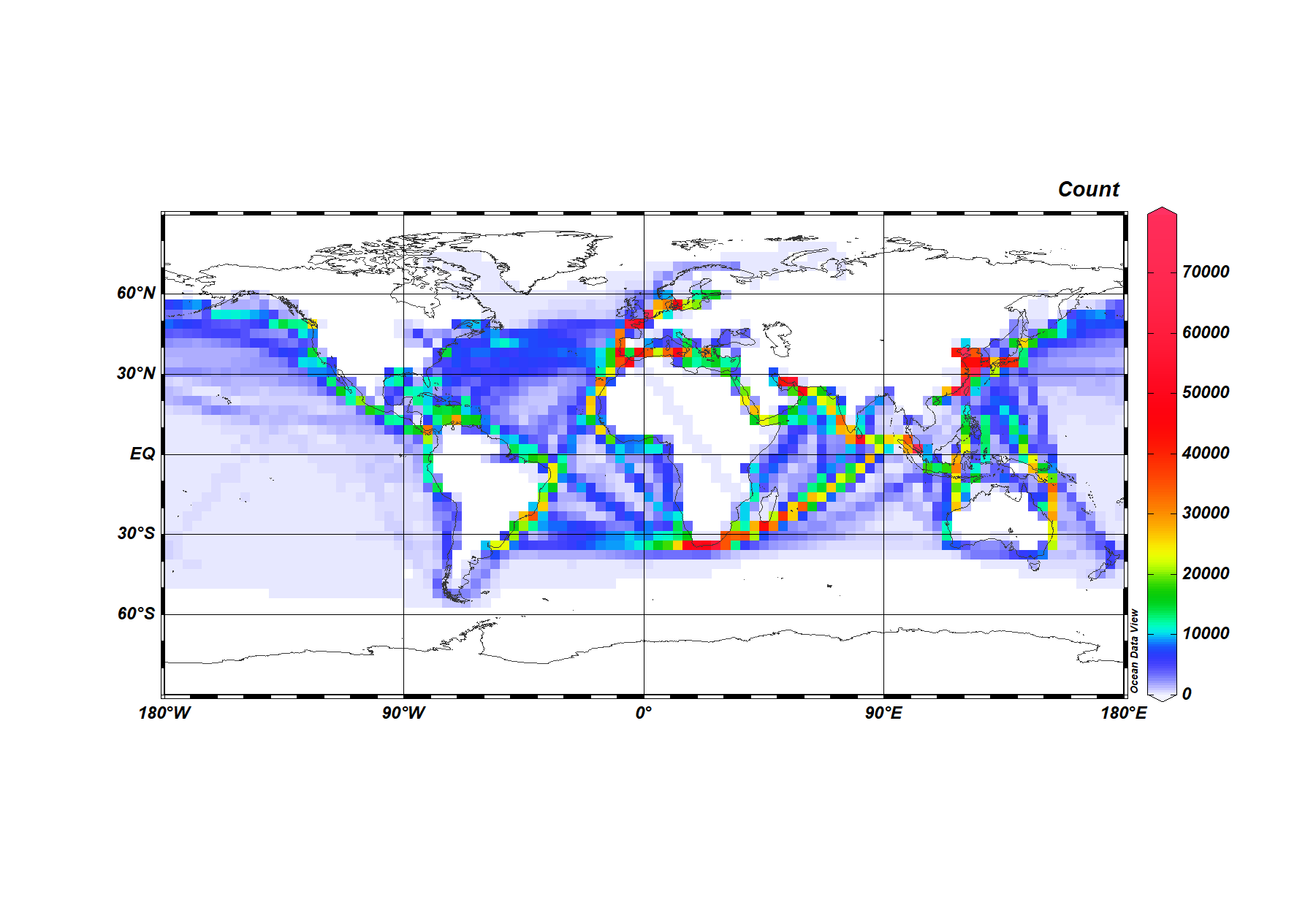
We make heat maps with all the documents: