Sums, series, and products in Diophantine approximation

Abstract

There is not much that can be said for all $x$ and for all $n$ about the sum

$$\sum _{k=1}^n\frac{1}{|\sin k\pi x|}.$$

However, for this and similar sums, series, and products, we can establish results for almost all $x$ using the tools of continued fractions. We present in detail the appearance of these sums in the singular series for the circle method. One particular interest of the paper is the detailed proof of a striking result of Hardy and Littlewood, whose compact proof, which delicately uses analytic continuation, has not been written freshly anywhere since its original publication. This story includes various parts of late 19th century and early 20th century mathematics.

1 Introduction

In this paper we survey a class of estimates for sums, series, and products that involve Diophantine approximation. We both sort out a timeline of the literature on these questions and give careful proofs of many lesser known results. Rather than being an open-pit mine for the history of Diophantine approximation, this paper follows one vein as deep as it goes.

For $x\in ℝ$, we write $\parallel x\parallel ={\min }_{n\in \mathbb{Z}}|x-n|$, the distance from $x$ to a nearest integer. In this paper we give a comprehensive presentation of estimates for sums whose $j$th term involves $\parallel jx\parallel$ and determine the abscissa of convergence and radius of convergence respectively of Dirichlet series and power series whose $j$th term involves $\parallel jx\parallel$. We also give a detailed proof of a result of Hardy and Littlewood that

$$\underset{n\to \mathrm{\infty }}{lim}{\left(\prod _{k=1}^n|\sin k\pi x|\right)}^{1/n}=\frac{1}{2}$$

for almost all $x$.

We either prove or state in detail and give references for all the material on continued fractions and measure theory that we use in this paper. Many of the results we prove in this paper do not have detailed proofs written in any books, and the proofs we give for results that do have proofs in books are often written significantly more meticulously here than anywhere else; in some cases the proofs in the literature are so sketchy that the proof we give is written from scratch, for example Lemma 9. Our presentation of Hardy and Littlewood’s estimate for ${\prod }_{k=1}^n|\sin \pi kx|$ makes clear exactly what results in Diophantine approximation one needs for the proof.

In the next section we introduce the Bernoulli polynomials, the Euler-Maclaurin summation formula, and Euler’s constant, which we shall use in a few places. Because the calculations are similar to what we do in the rest of this paper and because we want to be comfortable using Bernoulli polynomials, we work things out from scratch rather than merely stating results as known. In the section after that we summarize various problems that involve sums of the type we are talking about in this paper.

2 The Bernoulli polynomials, the Euler-Maclaurin summation formula, and Euler’s constant

For $k\ge 0$, the Bernoulli polynomial $B_k(x)$ is defined by

(1)

The Bernoulli numbers are $B_k=B_k(0)$, the constant terms of the Bernoulli polynomials. For any $x$, using L’Hospital’s rule the left-hand side of (1) tends to $1$ as $z\to 0$, and the right-hand side tends to $B_0(x)$, hence $B_0(x)=1$. Differentiating (1) with respect to $x$,

$$\sum _{k=0}^{\mathrm{\infty }}{B}_k^{\prime }(x)\frac{z^k}{k!}=\frac{z^2{e}^{xz}}{e^z-1}=\sum _{k=0}^{\mathrm{\infty }}{B}_k(x)\frac{z^{k+1}}{k!}=\sum _{k=1}^{\mathrm{\infty }}{B}_{k-1}(x)\frac{z^k}{(k-1)!},$$

so $B_0^{\prime }(x)=0$ and for $k\ge 1$ we have $\frac{B_k^{\prime }(x)}{k!}=\frac{B_{k-1}(x)}{(k-1)!}$, i.e.

$$B_k^{\prime }(x)=k{B}_{k-1}(x).$$

Furthermore, integrating (1) with respect to $x$ on $[0,1]$ gives, since $\int e^{xz}𝑑x=\frac{e^z-1}{z}$,

hence ${\int }_0^1{B}_0(x)𝑑x=1$ and for $k\ge 1$,

$${\int }_0^1{B}_k(x)𝑑x=0.$$

The first few Bernoulli polynomials are

$$B_0(x)=1,B_1(x)=x-\frac{1}{2},B_2(x)=x^2-x+\frac{1}{6},B_3(x)=x^3-\frac{3}{2}{x}^2+\frac{1}{2}x.$$

The Bernoulli polynomials satisfy the following:

${\displaystyle \sum _{k=0}^{\mathrm{\infty }}}{B}_k(x+1){\displaystyle \frac{z^k}{k!}}$ $={\displaystyle \frac{z{e}^{(x+1)z}}{e^z-1}}$

$={\displaystyle \frac{z{e}^{xz}(e^z-1+1)}{e^z-1}}$

$=z{e}^{xz}+{\displaystyle \frac{z{e}^{xz}}{e^z-1}}$

$={\displaystyle \sum _{k=0}^{\mathrm{\infty }}}{\displaystyle \frac{x^k{z}^{k+1}}{k!}}+{\displaystyle \sum _{k=0}^{\mathrm{\infty }}}{B}_k(x){\displaystyle \frac{z^k}{k!}}$

$={\displaystyle \sum _{k=1}^{\mathrm{\infty }}}{\displaystyle \frac{x^{k-1}{z}^k}{(k-1)!}}+{\displaystyle \sum _{k=0}^{\mathrm{\infty }}}{B}_k(x){\displaystyle \frac{z^k}{k!}},$

hence

$$B_k(x+1)=k{x}^{k-1}+B_k(x),k\ge 1,x\in ℝ.$$ (2)

In particular, for $k\ge 2$, $B_k(1)=B_k(0)$. The identity (2) yields Faulhaber’s formula, for $k\ge 0$ and positive integers ,

$$\sum _{a\le m\le b}{m}^k=\frac{B_{k+1}(b+1)-B_{k+1}(a)}{k+1}.$$ (3)

The following identity is the multiplication formula for the Bernoulli polynomials, found by Raabe [122, pp. 19–24, §13].

Lemma 1.

For $k\mathrm{\ge }\mathrm{0}$, $q\mathrm{\ge }\mathrm{1}$, and $x\mathrm{\in }ℝ$,

$$q{B}_k(qx)=q^k\sum _{j=0}^{q-1}{B}_k\left(x+\frac{j}{q}\right).$$

Proof.

Using (2) with $x=\frac{qn+j}{q}=n+\frac{j}{q}$,

$${(qn+j)}^k=\frac{q^k}{k+1}\left(B_{k+1}\left(n+\frac{j}{q}+1\right)-B_{k+1}\left(n+\frac{j}{q}\right)\right),$$

thus

${\displaystyle \sum _{m=q}^{Nq-1}}{m}^k$ $={\displaystyle \sum _{n=1}^{N-1}}{\displaystyle \sum _{j=0}^{q-1}}{(nq+j)}^k$

$={\displaystyle \frac{q^k}{k+1}}{\displaystyle \sum _{j=0}^{q-1}}{\displaystyle \sum _{n=1}^{N-1}}\left(B_{k+1}\left(n+{\displaystyle \frac{j}{q}}+1\right)-B_{k+1}\left(n+{\displaystyle \frac{j}{q}}\right)\right)$

$={\displaystyle \frac{q^k}{k+1}}{\displaystyle \sum _{j=0}^{q-1}}\left(B_{k+1}\left(N+{\displaystyle \frac{j}{q}}\right)-B_{k+1}\left(1+{\displaystyle \frac{j}{q}}\right)\right).$

Then by (3),

$$B_{k+1}(qN)-B_{k+1}(q)=q^k\sum _{j=0}^{q-1}\left(B_{k+1}\left(N+\frac{j}{q}\right)-B_{k+1}\left(1+\frac{j}{q}\right)\right).$$

Let $F_{k,q}(x)=B_{k+1}(qx)-q^k{\sum }_{j=0}^{q-1}{B}_{k+1}(x+j/q)$, which is a polynomial of degree $\le k+1$. The above means that for $N\ge 1$, $F_{k,q}(N)=F_{k,q}(1)$, which implies that the polynomial $F_{k,q}(x)-F_{k,q}(1)$ is identically $0$ and, a fortiori, $F_{k,q}^{\prime }(x)$ is identically $0$:

$$q{B}_{k+1}^{\prime }(qx)-q^k\sum _{j=0}^{q-1}{B}_{k+1}^{\prime }\left(x+\frac{j}{q}\right)=0.$$

Using $B_{k+1}^{\prime }(x)=(k+1)B_k(x)$,

$$q{B}_k(qx)=q^k\sum _{j=0}^{q-1}{B}_k\left(x+\frac{j}{q}\right).$$

∎

We remark that for prime $p$ and for $k\ge 0$, one uses Lemma 1 to prove that there is a unique $p$-adic distribution ${\mu }_{B,k}$ on the $p$-adic integers ${\mathbb{Z}}_p$ such that ${\mu }_{B,k}(a+p^N{\mathbb{Z}}_p)=p^{N(k-1)}{B}_k(a/p^N)$ [80, p. 35, Chapter II, §4], called a Bernoulli distribution.

For $x\in ℝ$, let $[x]$ be the greatest integer $\le x$, and let $R(x)=x-[x]$, called the fractional part of $x$. Write $𝕋=ℝ/\mathbb{Z}$ and define the periodic Bernoulli functions $P_k:𝕋\to ℝ$ by

$$P_k=B_k\circ R.$$

For $k\ge 2$, because $B_k(1)=B_k(0)$, the function $P_k$ is continuous. For $f:𝕋\to ℂ$ define its Fourier series $\widehat{f}:\mathbb{Z}\to ℂ$ by

$$\widehat{f}(n)={\int }_{𝕋}f(t)e^{-2\pi int}𝑑t,n\in \mathbb{Z}.$$

For $k\ge 1$, one calculates ${\widehat{P}}_k(0)=0$ and using integration by parts, ${\widehat{P}}_k(n)=-\frac{1}{{(2\pi in)}^k}$ for $n\ne 0$. Thus for $k\ge 1$, the Fourier series of $P_k$ is

$$P_k(t)\sim \sum _{n\in \mathbb{Z}}{\widehat{P}}_k(n)e^{2\pi int}=-\frac{1}{{(2\pi i)}^k}\sum _{n\ne 0}{n}^{-k}{e}^{2\pi int}.$$

For $k\ge 2$, , from which it follows that ${\sum }_{|n|\le N}{\widehat{P}}_k(n)e^{2\pi int}$ converges to $P_k(t)$ uniformly for $t\in 𝕋$. Furthermore, for $t\notin \mathbb{Z}$ [102, p. 499, Theorem B.2],

$$P_1(t)=-\frac{1}{\pi }\sum _{n=1}^{\mathrm{\infty }}\frac{1}{n}\sin 2\pi nt.$$

Thus for example,

$$B_1\left(\frac{1}{2\pi }\right)=P_1\left(\frac{1}{2\pi }\right)=-\frac{1}{\pi }\sum _{k=1}^{\mathrm{\infty }}\frac{\sin k}{k}.$$

The Euler-Maclaurin summation formula is the following [102, p. 500, Theorem B.5]. If are real numbers, $K$ is a positive integer, and $f$ is a $C^K$ function on an open set that contains $[a,b]$, then

$={\displaystyle {\int }_a^b}f(x)𝑑x+{\displaystyle \sum _{k=1}^K}{\displaystyle \frac{{(-1)}^k}{k!}}(P_k(b)f^{(k-1)}(b)-P_k(a)f^{(k-1)}(a))$

$-{\displaystyle \frac{{(-1)}^K}{K!}}{\displaystyle {\int }_a^b}{P}_K(x)f^{(K)}(x)𝑑x.$

Applying the Euler-Maclaurin summation formula with $a=1,b=n,K=2,f(x)=\log x$ yields [102, p. 503, Eq. B.25]

$$\sum _{1\le m\le n}\log n=n\log n-n+\frac{1}{2}\log n+\frac{1}{2}\log 2\pi +O(n^{-1}).$$

Using $e^{1+O(n^{-1})}=1+O(n^{-1})$, taking the exponential of the above equation gives Stirling’s approximation,

$$n!=n^n{e}^{-n}\sqrt{2\pi n}(1+O(n^{-1})).$$

Write $a_n=-\log n+{\sum }_{1\le m\le n}\frac{1}{m}$. Because $x\mapsto \log (1-x)$ is concave,

$$a_n-a_{n-1}=\frac{1}{n}+\log \left(1-\frac{1}{n}\right)\le 1+1-\frac{1}{n}=0,$$

which means that the sequence $a_n$ is nonincreasing. For $f(x)=\frac{1}{x}$, because $f$ is positive and nonincreasing,

$$\sum _{1\le m\le n}f(m)\ge {\int }_1^{n+1}f(x)𝑑x=\log (n+1)>\log n,$$

hence $a_n>0$. Because the sequence $a_n$ is positive and nonincreasing, there exists some nonnegative limit, $\gamma$, called Euler’s constant. Using the Euler-Maclaurin summation formula with $a=1,b=n,K=1,f(x)=\frac{1}{x}$, as $P_1(x)=[x]-\frac{1}{2}$,

which is

As $0\le R(x)x^{-2}\le x^{-2}$, the function $x\mapsto R(x)x^{-2}$ is integrable on $[1,\mathrm{\infty })$; let $C=1-{\int }_1^{\mathrm{\infty }}R(x)x^{-2}$. Since $0\le {\int }_n^{\mathrm{\infty }}R(x)x^{-2}𝑑x\le {\int }_n^{\mathrm{\infty }}{x}^{-2}𝑑x=n^{-1}$,

$$\sum _{1\le m\le n}\frac{1}{m}=\log n+C+O(n^{-1})$$

f. But $-\log n+{\sum }_{1\le m\le n}\frac{1}{m}\to \gamma$ as $n\to \mathrm{\infty }$, from which it follows that $C=\gamma$ and thus

$$\sum _{1\le m\le n}\frac{1}{m}=\log n+\gamma +O(n^{-1}).$$

3 Background

For $x\in ℝ$, let $[x]$ be the greatest integer $\le x$ and let $R(x)=x-[x]$. It will be handy to review some properties of $x\mapsto [x]$. For $n\in \mathbb{Z}$ it is immediate that $[x+n]=[x]$. For $x,y\in ℝ$ we have , which means , and using $[x+n]=[x]$ this is , therefore

$$[x]+[y]\le [x+y]\le [x]+[y]+1.$$

For $m,n\in \mathbb{Z}$, $n>1$, and $x\in ℝ$,

$$\left[\frac{x+m}{n}\right]=\left[\frac{[x]+m}{n}\right].$$

For $n$ a positive integer and for real $x$,

$$[x]=\left[x+\frac{0}{n}\right]\le \left[x+\frac{1}{n}\right]\le \mathrm{\cdots }\left[x+\frac{n-1}{n}\right]\le \left[x+\frac{n}{n}\right]=[x]+1.$$

There is a unique $\nu$, $1\le \nu \le n$, such that $\left[x+\frac{\nu -1}{n}\right]=[x]$ and $\left[x+\frac{\nu }{n}\right]=[x]+1$, and therefore $\left[R(x)+\frac{\nu -1}{n}\right]=0$ and $\left[R(x)+\frac{\nu }{n}\right]=1$, consequently and $R(x)+\frac{\nu }{n}\ge 1$, which means , from which finally we get and so $n=[nx]-n[x]+\nu$. But

$$\sum _{k=0}^{n-1}\left[x+\frac{k}{n}\right]=\sum _{k=0}^{\nu -1}[x]+\sum _{k=\nu }^{n-1}([x]+1)=\nu [x]+(n-\nu )([x]+1)=n[x]+n-\nu ,$$

and using $\nu =n-[nx]+n[x]$,

$$\sum _{k=0}^{n-1}\left[x+\frac{k}{n}\right]=n[x]+n-(n-[nx]+n[x])=[nx].$$

This identity is proved by Hermite [65, pp. 310–315, §V].

The Legendre symbol is defined in the following way. Let $p$ be an odd prime, and let $a$ be an integer that is not a multiple of $p$. If there is an integer $b$ such that $a\equiv b^2(modp)$ then $\left(\frac{a}{p}\right)=1$, and otherwise $\left(\frac{a}{p}\right)=-1$. In other words, for an integer $a$ that is relatively prime to $p$, if $a$ is a square mod $p$ then $\left(\frac{a}{p}\right)=1$, and if $a$ is not a square mod $p$ then $\left(\frac{a}{p}\right)=-1$. For example, one checks that there is no integer $b$ such that $b^2\equiv 6(mod7)$, and hence $\left(\frac{6}{7}\right)=-1$, while $3^2\equiv 2(mod7)$, and so $\left(\frac{2}{7}\right)=1$.

If $p$ and $q$ are distinct odd primes, define integers $u_k$, $1\le k\le \frac{p-1}{2}$, by

$$kq=p\left[\frac{kq}{p}\right]+u_k;$$

namely, $u_k$ is the remainder of $kq$ when divided by $p$. We have $1\le u_k\le p-1$. Let $\mu (q,p)$ be the number of $k$ such that $u_k>\frac{p-1}{2}$. It can be shown that [59, p. 74, Theorem 92]

$$\left(\frac{q}{p}\right)={(-1)}^{\mu (q,p)};$$

this fact is called Gauss’s lemma. For example, for $p=13$ and $q=3$ we work out that

$$u_1=3,u_2=6,u_3=9,u_4=12,u_5=2,u_6=5,$$

and hence $\mu (3,13)=2$, so ${(-1)}^{\mu (3,13)}=1$; on the other hand, $4^2\equiv 3(mod13)$, hence $\left(\frac{3}{13}\right)=1$. With

$$S(q,p)=\sum _{j=1}^{\frac{p-1}{2}}\left[\frac{jq}{p}\right],$$

it is known that [59, pp. 77-78, §6.13]

$$S(q,p)\equiv \mu (q,p)(mod2).$$

And it can be shown that [59, p. 76, Theorem 100]

$$S(q,p)+S(p,q)=\frac{p-1}{2}\cdot \frac{q-1}{2}.$$ (4)

Thus

$\left({\displaystyle \frac{p}{q}}\right)\left({\displaystyle \frac{q}{p}}\right)$ $=$ ${(-1)}^{\mu (p,q)+\mu (q,p)}$

$=$ ${(-1)}^{S(p,q)+S(q,p)}$

$=$ ${(-1)}^{\frac{p-1}{2}\cdot \frac{q-1}{2}}.$

This is Gauss’s third proof of the law of quadratic reciprocity in the numbering [7, p. 50, §20]. This proof was published in Gauss’s 1808 “Theorematis arithmetici demonstratio nova”, which is translated in [140, pp. 112–118]. Dirichlet [38, pp. 65–72, §§42–44] gives a presentation of the proof. Eisenstein’s streamlined version of Gauss’s third proof is presented with historical remarks in [93]. Lemmermeyer [95] gives a comprehensive history of the law of quadratic reciprocity, and in particular writes about Gauss’s third proof [95, pp. 9–10]. The formula (4) resembles the reciprocity formula for Dedekind sums [123, p. 4, Theorem 1].

Gauss obtains (4) from the following [140, p. 116, §5]: if $x$ is irrational and $n$ is a positive integer, then

$$\sum _{k=1}^n[kx]+\sum _{k=1}^{[nx]}\left[\frac{k}{x}\right]=n[nx],$$ (5)

which he proves as follows. If , then $[kx]=j$. Therefore

${\displaystyle \sum _{k=1}^n}[kx]$ $=$ ${\displaystyle \sum _{j=1}^{[nx]}}j\left(\left[{\displaystyle \frac{j+1}{x}}\right]-\left[{\displaystyle \frac{j}{x}}\right]\right)$

$=$ $n[nx]-{\displaystyle \sum _{j=1}^{[nx]}}\left[{\displaystyle \frac{j}{x}}\right].$

Bachmann [6, pp. 654–658, §4] surveys later work on sums similar to (5); see also Dickson [35, Chapter X]. If $m$ and $n$ are relatively prime, then

$$\{R\left(\frac{m}{n}\right),R\left(\frac{2m}{n}\right),\mathrm{\dots },R\left(\frac{(n-1)m}{n}\right)\}=\{\frac{1}{n},\frac{2}{n},\mathrm{\dots },\frac{n-1}{n}\},$$

and so

$$\sum _{k=1}^{n-1}R\left(\frac{km}{n}\right)=\sum _{k=1}^{n-1}\frac{k}{n}=\frac{1}{n}\cdot \frac{(n-1)n}{2}=\frac{n-1}{2}.$$

Hence

$$\sum _{k=1}^{n-1}\left[\frac{km}{n}\right]=\sum _{k=1}^{n-1}\frac{km}{n}-\sum _{k=1}^{n-1}R\left(\frac{km}{n}\right)=\frac{(m-1)(n-1)}{2}.$$ (6)

There is also a simple lattice point counting argument [118, p. 113, No. 18] that gives (6).

In 1849, Dirichlet [37] shows that

$$\sum _{k=1}^{n}d(k)=\sum _{k=1}^n\left[\frac{n}{k}\right],$$

where $d(n)$ denotes the number of positive divisors of an integer $n$. (This equality is Dirichlet’s “hyperbola method”.) He then proves that

$$\sum _{k=1}^n\left[\frac{n}{k}\right]=n\log n+(2\gamma -1)n+O(\sqrt{n}).$$

Hardy and Wright [59, pp. 264–265, Theorem 320] give a proof of this. Finding the best possible error term in the estimate for ${\sum }_{k=1}^{n}d(k)$ is “Dirichlet’s divisor problem”. Dirichlet cites the end of Section V Gauss’s Disquisitiones Arithmeticae as precedent for determining average magnitudes of arithmetic functions. (In Section V, Articles 302–304, of the Disquisitiones Arithmeticae, Gauss writes about averages of class numbers of binary quadratic forms, cf. [36, Chapter VI].)

Define $(x)$ to be $0$ if $x\in \mathbb{Z}+\frac{1}{2}$; if $x\notin \mathbb{Z}+\frac{1}{2}$ then there is an integer $m_x$ for which for all integers $n\ne m_x$, and we define $(x)$ to be $x-m_x$. Riemann [125, p. 105, §6] defines

$$f(x)=\sum _{n=1}^{\mathrm{\infty }}\frac{(nx)}{n^2};$$

for any $x$, the series converges absolutely because . Riemann states that if $p$ and $m$ are relatively prime and $x=\frac{p}{2m}$, then

$$f(x^{+})=\underset{h\to 0^{+}}{lim}f(x+h)=f(x)-\frac{{\pi }^2}{16m^2},f(x^{-})=\underset{h\to 0^{-}}{lim}f(x+h)=f(x)+\frac{{\pi }^2}{16m^2},$$

thus

$$f(x^{-})-f(x^{+})=\frac{{\pi }^2}{8m^2},$$

and hence that $f$ is discontinuous at such points, and says that at all other points $f$ is continuous; see Laugwitz [94, §2.1.1, pp. 183-184], Neuenschwander [108], and Pringsheim [119, p. 37] about Riemann’s work on pathological functions. The role of pathological functions in the development of set theory is explained by Dauben [32, Chapter 1, p. 19] and Ferreirós [49, Chapter V, §1, p. 152].

For any interval $[a,b]$ and any $\sigma >0$, it is apparent from the above that there are only finitely many $x\in [a,b]$ for which $f(x^{-})-f(x^{+})>\sigma$, and Riemann deduces from this that $f$ is Riemann integrable on $[a,b]$; cf. Hawkins [63, p. 18] on the history of Riemann integration. Later in the same paper [125, p. 129, §13], Riemann states that the function

$$x\mapsto \sum _{n=1}^{\mathrm{\infty }}\frac{(nx)}{n},$$

is not Riemann integrable in any interval.

In 1897, Cesàro [28] asks the following question (using the pseudonym, and anagram, “Rosace” [112, p. 331]). Let $ϵ(x)=x-[x]-\frac{1}{2}$. Is the series

$$\sum _{n=1}^{\mathrm{\infty }}\frac{ϵ(nx)}{n}$$ (7)

convergent for all non-integer $x$? This is plausible because the expected value of $ϵ(x)$ is 0. Landau [89] answers this question in 1901. Landau proves that if there is some $g$ such that

$$\sum _{k=1}^n[kx]=\frac{n(n+1)x}{2}-\frac{n}{2}+O(g(n))$$

where $g$ is a nonnegative function such $g(n)=o(n)$ and such that ${\sum }_{n=1}^{\mathrm{\infty }}\frac{g(n)}{n(n+1)}$ converges, then (7) converges. And he proves that if $x$ is rational then (7) diverges. We return to this series in §9.

Also in 1898, Franel [52] asks whether for irrational $x$ and for $ϵ>0$ we have

$$\sum _{k=1}^n[kx]=\frac{n(n+1)x}{2}-\frac{n}{2}+O(n^{ϵ}).$$

Then in 1899, Franel [53] asks if we can do better than this: is the error term in fact $O(1)$? Cesàro and Franel each contributed many problems to L’Intermédiaire des mathématiciens, the periodical in which they posed their questions. Information about Franel is given in [82].

Lerch [96] answers Franel’s questions in 1904. If $x$ is irrational and $\frac{p}{q}$ is a convergent of $x$ (which we will define in §4), then using Theorem 2 (from §4) we can show that if $1\le k\le q$ then $[kx]=[\frac{kp}{q}]$. Lerch uses this and (6) to show that if $x$ is irrational and $\frac{p}{q}$ is a convergent of $x$ then

Lerch states that if the continued fraction expansion of $x$ has bounded partial quotients (defined in §4) then, for any positive integer $n$,

$$\sum _{k=1}^n[kx]=\frac{n(n+1)x}{2}-\frac{n}{2}+O(\log n).$$

Lerch only gives a brief indication of the proof of this. This result is proved by Hardy and Littlewood in 1922 [57, p. 24, Theorem B3], and also in 1922 by Ostrowski [110, p. 81]. On the other hand, Lerch also constructs examples of $x$ such that, for some positive integer $c$,

$$\left|\sum _{k=1}^n[kx]-\frac{n(n+1)x}{2}+\frac{n}{2}\right|\gg n^{1-\frac{1}{c}}.$$

Nevertheless, in 1909 Sierpinski [135] proves that if $x$ is irrational then

$$\sum _{k=1}^n[kx]=\frac{n(n+1)x}{2}-\frac{n}{2}+o(n).$$

A bibliography of Lerch’s works is given in [139]. Lerch had written earlier papers on Gauss sums, Fourier series, theta functions, and the class number; many of his papers are in Czech, but some of them are in French, several of which were published in the Paris Comptes rendus. Several of Lerch’s papers are discussed in Cresse’s survey of the class number of binary quadratic forms [36, Chapter VI].

In 1899, a writer using the pseudonym “Quemquaeris” [121] (“quem quaeris” = “whom you seek”) asks if we can characterize $\varphi (n)$ such that for all irrational $\theta$ the series

$$\sum _{n=1}^{\mathrm{\infty }}\frac{\varphi (n)}{\sin n\pi \theta }$$

converges. In particular, the writer asks if $\varphi (n)=\frac{1}{n!}$ satisfies this. In the same year, de la Vallée-Poussin [34] answers this question. (There are also responses following de la Vallée-Poussin’s by Borel and Fabry.) For a given function $\varphi (n)$, de la Vallée-Poussin shows that if we have $a_n>\frac{1}{\varphi (q_{n-1})}$ for all $n$, for $a_n$ the $n$th partial quotient of $\theta$ and $q_n$ the denominator of the $n$th convergent of $\theta$, then the series

$$\sum _{n=1}^{\mathrm{\infty }}\frac{\varphi (n)}{\sin n\pi \theta }$$

will diverge. Hardy and Littlewood prove numerous results on similar series, e.g. for $\varphi (n)=n^{-r}$ for real $r>1$ and for certain classes of $\theta$, in their papers on Diophantine approximation [61]. In 1931, Walfisz [152, p. 570, Hilfssatz 4] shows, following work of Behnke [13, p. 289, §16], that for almost all irrational $x\in [0,1]$, if $ϵ>0$ then

$$\sum _{k=1}^n\frac{1}{\parallel k\theta \parallel }=O(n{(\log n)}^{2+ϵ}),$$

where $\parallel x\parallel =\min (R(x),1-R(x))$. Walfisz’s paper includes many results on related sums.

In 1916, Watson [153] finds the following asymptotic series for $S_n={\sum }_{m=1}^{n-1}\csc \left(\frac{m\pi }{n}\right)$:

$$\pi S_n\sim 2n\log (2n)+2n(\gamma -\log \pi )+\sum _{j=1}^{\mathrm{\infty }}{(-1)}^j\frac{B_{2j}^2(2^{2j}-2){\pi }^{2j}}{j(2j)!n^{2j-1}},$$

where $\gamma$ is Euler’s constant and $B_j$ are the Bernoulli numbers. Truncating the asymptotic series and rewriting gives

$$S_n=\frac{2n\log n}{\pi }+n\cdot \frac{2\log 2+2\gamma -2\log \pi }{\pi }+O\left(\frac{1}{n}\right).$$

For example, computing $S_{1000}$ directly we get $S_{1000}=4477.593932\mathrm{\dots }$, and computing the right-hand side of the above formula without the error term we obtain $4477.594019\mathrm{\dots }$ A cleaner derivation of the asymptotic series using the Euler-Maclaurin summation formula is given later by Williams [155].

Early surveys of Diophantine approximation are given by Bohr and Cramér [20, pp. 833–836, §39] and Koksma [81, pp. 102–110]. Hlawka and Binder [66] present the history of the initial years of the theory of uniform distribution. Narkiewicz [106, pp. 82–95, §2.5 and pp. 175–183 §3.5] gives additional historical references on Diophantine approximation. The papers of Hardy and Littlewood on Diophantine approximation are reprinted in [61]. Perron [113] and Brezinski [23] give historical references on continued fractions, and there is reliable material on the use of continued fractions by 17th century mathematicians in Whiteside [154]. Fowler [51] presents a prehistory of continued fractions in Greek mathematics.

4 Preliminaries on continued fractions

Let

$$\parallel x\parallel =\underset{k\in \mathbb{Z}}{\min }|x-k|=\min (R(x),1-R(x)).$$

Let $\mu$ be Lebesgue measure on $[0,1]$, and let $\mathrm{\Omega }=[0,1]\setminus \mathbb{Q}$.

For positive integers $a_1,\mathrm{\dots },a_n$, we define

$$[a_1,\mathrm{\dots },a_n]=\frac{1}{a_1+{\displaystyle \frac{1}{\mathrm{\cdots }+{\displaystyle \frac{1}{a_{n-1}+{\displaystyle \frac{1}{a_n}}}}}}}.$$

For example, $[1,1,1]=\frac{2}{3}$.

Let $\mathbb{N}$ be the set of positive integers. We call $a\in {\mathbb{N}}^{\mathbb{N}}$ a continued fraction, and we call $a_n$ the $n$th partial quotient of $a$. If there is some $K>0$ such that $a_n\le K$ for all $n$ then we say that $a$ has bounded partial quotients. We call $[a_1,\mathrm{\dots },a_n]$ the $n$th convergent of $a$. For $n\ge 1$ let

$$\frac{p_n}{q_n}=[a_1,\mathrm{\dots },a_n],$$

with $p_n,q_n$ positive integers that are relatively prime, and set

$$p_0=0,q_0=1.$$

One can show by induction [44, p. 70, Lemma 3.1] that for $n\ge 1$ we have

(8)

We have

$$p_1=1,q_1=a_1,$$

and from (8) we get for all $n\ge 1$ that

$$p_{n+1}=a_{n+1}{p}_n+p_{n-1},$$

and

$$q_{n+1}=a_{n+1}{q}_n+q_{n-1}.$$

Since the $a_n$ are positive integers we get by induction that for all $n\ge 1$,

$$p_n\ge 2^{(n-1)/2},q_n\ge 2^{(n-1)/2}.$$ (9)

In fact, setting $F_1=1,F_2=1$, $F_{n+1}=F_n+F_{n-1}$ for $n\ge 2$, with $F_n$ the $n$th Fibonacci number, as $a_n\ge 1$ we check by induction that

$$p_n\ge F_n,q_n\ge F_{n+1}.$$

Taking determinants of (8) gives us for all $n\ge 1$ that

$$p_n{q}_{n-1}-p_{n-1}{q}_n={(-1)}^{n+1},$$ (10)

and then by induction we have for all $n\ge 1$,

$$\frac{p_n}{q_n}=\sum _{k=1}^n\frac{{(-1)}^{k+1}}{q_{k-1}{q}_k}.$$

For any $a\in {\mathbb{N}}^{\mathbb{N}}$, as $n\to \mathrm{\infty }$ this sequence of sums converges and we denote its limit by $v(a)$. We have for all $n\ge 1$,

$$v(a)-\frac{p_n}{q_n}=\sum _{k=n+1}^{\mathrm{\infty }}\frac{{(-1)}^{k+1}}{q_{k-1}{q}_k}.$$

Since the right hand side is an alternating series we obtain for $n\ge 1$,

(11)

and

$$\left|v(a)-\frac{p_n}{q_n}\right|>\frac{1}{q_n{q}_{n+1}}-\frac{1}{q_{n+1}{q}_{n+2}}=\frac{a_{n+2}}{q_n{q}_{n+2}}\ge \frac{1}{q_n(q_{n+1}+q_n)},$$ (12)

and

(13)

For $x\in \mathrm{\Omega }$, we say that $\frac{p}{q}\in \mathbb{Q}$, $q>0$, is a best approximation to $x$ if $\parallel qx\parallel =|qx-p|$ and $\parallel q^{\prime }x\parallel >\parallel qx\parallel$ for . The following theorem shows in particular that the convergents of a continued fraction $a$ are best approximations to $v(a)$ [127, p. 22, Chapter 2, §3, Theorem 1].

Theorem 2 (Best approximations).

Let $a\mathrm{\in }{\mathbb{N}}^{\mathbb{N}}$. For any $n\mathrm{\ge }\mathrm{1}$,

$$\parallel q_{n}v(a)\parallel =|p_n-q_{n}v(a)|.$$

If , then for any $p\mathrm{\in }\mathbb{Z}$,

$$|qv(a)-p|\ge |p_n-q_{n}v(a)|.$$

Proof.

By (11), . But

$$q_{n+1}\ge q_2=a_2{q}_1+q_0\ge q_1+q_0=a_1+1\ge 2.$$

So , which means $\parallel q_{n}v(a)\parallel =|q_{n}v(a)-p_n|$.

Write $x=v(a)$ and let . Applying (10),

$$detA=p_{n+1}{q}_n-p_n{q}_{n+1}={(-1)}^n.$$

Let

Then

$$qx-p=(\mu q_{n+1}+\nu q_n)x-(p_{n+1}\mu +p_n\nu )=\mu (q_{n+1}x-p_{n+1})+\nu (q_{n}x-p_n)$$

and

In particular, $\mu ,\nu \in \mathbb{Z}$. Suppose by contradiction that $\nu =0$. Then $(q-\mu q_{n+1})x=p-\mu p_{n+1}$, and as $x\notin \mathbb{Q}$ it must then be that $q=\mu q_{n+1}$ and $p=\mu p_{n+1}$. But $q=\mu q_{n+1}$, , and $\mu \in \mathbb{Z}$ are together a contradiction. Therefore $\nu \ne 0$. Either $\mu =0$ or $\mu \ne 0$. For $\mu =0$,

$$|qx-p|=|\nu ||q_{n}x-p_n|\ge |q_{n}x-p_n|,$$

which is the claim. For $\mu \ne 0$ we use the fact $q=q_{n+1}\mu +q_n\nu$ and . If $\mu ,\nu >0$ then is contradicted, and if then $q\ge 1$ is contradicted. Therefore $\mu$ and $\nu$ have different signs, say $\mu ={(-1)}^N|\mu |$ and $\nu ={(-1)}^{N+1}|\nu |$. Furthermore, we get from (13) that

$$\mathrm{sgn}(q_{n}x-p_n)={(-1)}^n,\mathrm{sgn}(q_{n+1}x-p_{n+1})={(-1)}^{n+1}.$$

Therefore

$qx-p$ $=\mu (q_{n+1}x-p_{n+1})+\nu (q_{n}x-p_n)$

$={(-1)}^N|\mu |\cdot {(-1)}^{n+1}|q_{n+1}x-p_{n+1}|+{(-1)}^{N+1}|\nu |\cdot {(-1)}^n|q_{n}x-p_n|,$

hence

$$|qx-p|=|\mu ||q_{n+1}x-p_{n+1}|+|\nu ||q_{n}x-p_n|\ge |\nu ||q_{n}x-p_n|\ge |q_{n}x-p_n|,$$

which is the claim. ∎

The above theorem says, a fortiori, that the convergents of $a$ are best approximations to $v(a)$. It can also be proved that if $\frac{p}{q}\in \mathbb{Q}$, $q>0$, is a best approximation to $v(a)$ then $\frac{p}{q}$ is a convergent of $a$ [92, p. 9, Theorem 6]. Cassels [27, p. 2, Chapter I] works out the theory of continued fractions according to this point of view. Similarly, Milnor [101, p. 234, Appendix C] works out the theory of continued fractions in the language of rotations of the unit circle.

We define the Gauss transformation $T:\mathrm{\Omega }\to \mathrm{\Omega }$ by $T(x)=R\left(\frac{1}{x}\right)$ for $x\in \mathrm{\Omega }$, and we define $\mathrm{\Phi }:\mathrm{\Omega }\to {\mathbb{N}}^{\mathbb{N}}$ by

$${(\mathrm{\Phi }(x))}_n=\left[\frac{1}{T^{n-1}(x)}\right],n\ge 1.$$

One can check that if $a\in {\mathbb{N}}^{\mathbb{N}}$ then $v(a)\in \mathrm{\Omega }$ [44, p. 73, Lemma 3.2]. (Namely, the value of a nonterminating continued fraction is irrational.) One can prove that $v:{\mathbb{N}}^{\mathbb{N}}\to \mathrm{\Omega }$ is injective [44, p. 75, Lemma 3.4], and for $x\in \mathrm{\Omega }$ that [44, p. 78, Lemma 3.6]

$$(v\circ \mathrm{\Phi })(x)=x.$$

Therefore $\mathrm{\Phi }:\mathrm{\Omega }\to {\mathbb{N}}^{\mathbb{N}}$ is a bijection. Moreover, $\mathrm{\Phi }$ is a homeomorphism, when $\mathbb{N}$ has discrete topology, ${\mathbb{N}}^{\mathbb{N}}$ has the product topology, and $\mathrm{\Omega }$ has the subspace topology inherited from $ℝ$ [44, p. 86, Exercise 3.2.2]. That ${\mathbb{N}}^{\mathbb{N}}$ and $\mathrm{\Omega }$ are homeomorphic can also be proved without using continued fractions [2, p. 106, Theorem 3.68]. In descriptive set theory, the topological space $𝒩={\mathbb{N}}^{\mathbb{N}}$ is called the Baire space, and the Alexandrov-Urysohn theorem states that $𝒩$ has the universal property that any nonempty Polish space that is zero-dimensional (there is a basis of clopen sets for the topology) and all of whose compact subsets have empty interior is homeomorphic to $𝒩$ [75, p. 37, Theorem 7.7]. Some of Baire’s work on $𝒩$ is described in [71, pp. 119–120] and [5, pp. 349, 372].

For $I=[0,1]$ and for $T:I\to I$, $T(x)=R(1/x)$ for $x>0$ and $T(0)=0$. For $k\ge 1$ let $I_k=(\frac{1}{k+1},\frac{1}{k})$, so if $x\in I_k$ then $T(x)=x^{-1}-k$. Then for $x\in I=[0,1]$,

$$T(x)=\sum _{k=1}^{\mathrm{\infty }}{1}_{I_k}(x)(x^{-1}-k).$$

For $S=\{0\}\cup \{k^{-1}:k\ge 1\}$, $I\setminus S={\bigcup }_{k\ge 1}{I}_k$, and for $x\in I\setminus S$,

$$T^{\prime }(x)=-\sum _{k=1}^{\mathrm{\infty }}{1}_{I_k}(x)x^{-2},$$

and for $x\in I_k$, . Differentiability and dynamical properties of the Gauss transformation are worked out by Cornfeld, Fomin and Sinai [30, pp. 165–177, Chapter 7, §4], as an instance of piecewise monotonic transformations.

For each $n\ge 1$ we define $a_n:\mathrm{\Omega }\to \mathbb{N}$ by $a_n(x)={(\mathrm{\Phi }(x))}_n$. For example, $e-2\in \mathrm{\Omega }$, and it is known [92, p. 74, Theorem 2] that for $k\ge 1$,

$$a_{3k}(e-2)=a_{3k-2}(e-2)=1\mathit{\hspace{1em}}\text{and}\mathit{\hspace{1em}}{a}_{3k-1}(e-2)=2k.$$

The pattern for the continued fraction expansion of $e$ seems first to have been worked out by Roger Cotes in 1714 [50], and was later proved by Euler using a method involving the Riccati equation [31].

For $n\ge 1$ and $i\in {\mathbb{N}}^n$, let

$$I_n(i)=\{\omega \in \mathrm{\Omega }:a_k(x)=i_k,1\le k\le n\}.$$

For $x\in I_n(i)$,

$$\frac{p_n(x)}{q_n(x)}=[i_1,\mathrm{\dots },i_n],\frac{p_{n-1}(x)}{q_{n-1}(x)}=[i_1,\mathrm{\dots },i_{n-1}].$$

The following is an expression for the sets $I_n(i)$ [69, p. 18, Theorem 1.2.2].

Theorem 3.

Let $n\mathrm{\ge }\mathrm{1}$, $i\mathrm{\in }{\mathbb{Z}}_{\mathrm{\ge }\mathrm{1}}^n$, and for $p_n\mathrm{=}{p}_n\mathit{}\mathrm{(}x\mathrm{)}$, $q_n\mathrm{=}{q}_n\mathit{}\mathrm{(}x\mathrm{)}$, $x\mathrm{\in }{I}_n\mathit{}\mathrm{(}i\mathrm{)}$,

and

Then

$$I_n(i)=\mathrm{\Omega }\cap (u_n(i),v_n(i)).$$

It follows from the above that for $i\in {\mathbb{N}}^n$, $n\ge 1$,

$$\mu (I_n(i))=\frac{1}{q_n(q_n+q_{n-1})}.$$

5 Diophantine conditions

For real $\tau ,\gamma >0$ let

$𝒟(\tau ,\gamma )$ $={\displaystyle \bigcap _{q\in {\mathbb{Z}}_{\ge 1},p\in \mathbb{Z}}}\{x\in [0,1]:\left|x-{\displaystyle \frac{p}{q}}\right|\ge \gamma q^{-\tau }\}$

$={\displaystyle \bigcap _{q\in {\mathbb{Z}}_{\ge 1}}}\{x\in [0,1]:\parallel qx\parallel \ge \gamma q^{-\tau +1}\},$

and let

$$𝒟(\tau )=\bigcup _{\gamma >0}𝒟(\tau ,\gamma ).$$

We relate the sets $𝒟(\tau )$ and continued fractions expansions [101, p. 241, Lemma C.6], cf. [158, p. 130, Proposition 2.4].

Lemma 4.

For $\tau \mathrm{>}\mathrm{0}$ and $x\mathrm{\in }\mathrm{\Omega }$, $x\mathrm{\in }𝒟\mathit{}\mathrm{(}\tau \mathrm{)}$ if and only if there is some $C\mathrm{=}C\mathit{}\mathrm{(}x\mathrm{)}\mathrm{>}\mathrm{0}$ such that $q_{n\mathrm{+}\mathrm{1}}\mathit{}\mathrm{(}x\mathrm{)}\mathrm{\le }C\mathit{}{q}_n\mathit{}{\mathrm{(}x\mathrm{)}}^{\tau \mathrm{-}\mathrm{1}}$ for all $n\mathrm{\ge }\mathrm{1}$.

Proof.

For $x\in \mathrm{\Omega }$, write $q_n=q_n(x)$. By (12), $\parallel q_{n}x\parallel >\frac{1}{q_{n+1}+q_n}$, and by (11), . Suppose $x\in 𝒟(\tau )$, so there is some $\gamma >0$ such that $x\in 𝒟(\tau ,\gamma )$. Then

Suppose $q_{n+1}\le C{q}_n^{\tau -1}$ for all $n\ge 1$. For $q\in {\mathbb{Z}}_{\ge 1}$, take . Using Theorem 2,

$$\parallel qx\parallel \ge \parallel q_{n}x\parallel >\frac{1}{q_{n+1}+q_n}>\frac{1}{2q_{n+1}}\ge \frac{1}{2}{C}^{-1}{q}_n^{-\tau +1}\ge \frac{1}{2C}\cdot q^{-\tau +1},$$

which means that $x\in 𝒟(\tau ,\frac{1}{2C})$. ∎

For $K$ a positive integer, let

$${ℬ}_K=\{x\in \mathrm{\Omega }:a_n(x)\le K\text{ for all }n\ge 1\},$$

so $ℬ={\bigcup }_{K\ge 1}{ℬ}_K$ is the set of those $x\in \mathrm{\Omega }$ with bounded partial quotients.

Lemma 5.

For $x\mathrm{\in }\mathrm{\Omega }$, $x\mathrm{\in }𝒟\mathit{}\mathrm{(}\mathrm{2}\mathrm{)}$ if and only if $x\mathrm{\in }ℬ$.

Proof.

Write $a_n=a_n(x)$ and $q_n=q_n(x)$. If $x\in 𝒟(2)$ then there is some $\gamma >0$ such that $x\in 𝒟(2,\gamma )$, hence for $n\ge 1$,

Now, $q_{n+1}=a_{n+1}{q}_n+q_{n-1}$ for $n\ge 1$, so

which shows that $x$ has bounded partial quotients.

If $x\in {ℬ}_K$, let $q\in {\mathbb{Z}}_{\ge 1}$ and let . Using Theorem 2 and then (12),

$$\parallel qx\parallel \ge \parallel q_{n}x\parallel >\frac{1}{q_{n+1}+q_n}=\frac{1}{a_{n+1}{q}_n+q_{n-1}+q_n}>\frac{1}{(a_{n+1}+2)q_n}.$$

As $x\in {ℬ}_K$,

$$\parallel qx\parallel >\frac{1}{(K+2)q_n}\ge \frac{1}{K+2}{q}^{-1},$$

which means that $x\in 𝒟(2,\frac{1}{K+2})$. ∎

A complex number $\alpha$ is called an algebraic number of degree $d$, $d\ge 0$, if there is some polynomial $f\in \mathbb{Z}[x]$ with degree $d$ such that $f(\alpha )=0$ and if $g\in \mathbb{Z}[x]$ has degree and $g(\alpha )=0$ then $g=0$. An algebraic number number of degree $2$ is called a quadratic irrational. Let $\alpha \in \mathrm{\Omega }$. It was proved by Euler [59, p. 144, Theorem 176] that if there is some $p>0$ and some $L$ such that $a_{l+p}(\alpha )=a_l(\alpha )$ for all $l\ge L$ then $\alpha$ is a quadratic irrational The converse of this was proved by Lagrange [59, p. 144, Theorem 177], namely that a quadratic irrational has eventually periodic partial quotients. For example, $\alpha =\sqrt{11}-3\in \mathrm{\Omega }$ is a quadratic irrational, being a root of $x^2+6x-2$, and one works out that $a_1(\alpha )=3,a_2(\alpha )=6$, and that $a_{l+2}(\alpha )=a_l(\alpha )$ for $l\ge 1$. In particular, if $\alpha \in \mathrm{\Omega }$ is a quadratic irrational, then $\alpha$ has bounded partial quotients.

Liouville [59, p. 161, Theorem 191] proved that if $x\in \mathrm{\Omega }$ is an algebraic number of degree $d\ge 2$, then $x\in 𝒟(d)$. The Thue-Siegel-Roth theorem [48, p. 55, Theorem 1.23] states that if $x\in \mathrm{\Omega }$ is an algebraic number, then for any $\delta >0$ there is some $q_{\delta }\in {\mathbb{Z}}_{\ge 1}$ such that for all $q\ge q_{\delta }$,

$$\parallel qx\parallel \ge q^{-1-\delta }.$$

See Schmidt [131, p. 195, Theorem 2B].

6 Sums of reciprocals

We are interested in getting bounds on the sum ${\sum }_{j=1}^m\frac{1}{\parallel jx\parallel }$. This is an appealing question because the terms $\frac{1}{\parallel jx\parallel }$ are unbounded.

Rather than merely stating that ${\sum }_{k=1}^{\mathrm{\infty }}\frac{1}{k}=\mathrm{\infty }$, we give more information by giving the estimate

$$\sum _{k=1}^n\frac{1}{k}=\log n+\gamma +O(n^{-1}),$$

where $\gamma$ is Euler’s constant. Likewise, rather than merely stating that there are infinitely many primes, we state more information with [90, p. 102, §28]

$$\sum _{p\le x}\frac{1}{p}=\log \log x+B+O\left(\frac{1}{\log x}\right),$$

for a certain constant $B$ (namely “Merten’s constant”), or with [90, p. 226, §61]

$$\sum _{p\le x}p=\frac{x^2}{2\log x}+O\left(\frac{x^2}{{(\log x)}^2}\right).$$

Because $|\sin (\pi x)|=\sin (\pi \parallel x\parallel )\le \pi \parallel x\parallel$ and

$$|\sin (\pi x)|=\sin (\pi \parallel x\parallel )\ge \frac{2}{\pi }\pi \parallel x\parallel =2\parallel x\parallel ,$$

we have

$$\frac{1}{\pi }\sum _{j=1}^m\frac{1}{\parallel jx\parallel }\le \sum _{j=1}^m\frac{1}{|\sin \pi jx|}\le \frac{1}{2}\sum _{j=1}^m\frac{1}{\parallel jx\parallel }.$$ (14)

Thus, getting bounds on ${\sum }_{j=1}^m\frac{1}{\parallel jx\parallel }$ will give us bounds on ${\sum }_{j=1}^m\frac{1}{|\sin \pi jx|}$.

Let $\psi$ be a nondecreasing function defined on the positive integers such that $\psi (h)>0$ for $h\ge 1$ (for example, $\psi (h)=\log (2h)$). Following Kuipers and Niederreiter [85, p. 121, Definition 3.3], we say that an irrational number $x$ is of type if $\parallel hx\parallel \ge \frac{1}{h\psi (h)}$ for all integers $h\ge 1$. If $\psi$ is a constant function, then we say that $x$ is of constant type.

Lemma 6.

$x\in \mathrm{\Omega }$ is of constant type if and only if it has bounded partial quotients.

Proof.

Suppose that $x\in \mathrm{\Omega }$ is of constant type. So there is some $K>0$ such that $\parallel hx\parallel \ge \frac{1}{hK}$ for all integers $h\ge 1$. For $n\ge 2$ we have $q_n=a_n{q}_{n-1}+q_{n-2}$, and hence, by (11),

showing that $x$ has bounded partial quotients.

Suppose that $x\in \mathrm{\Omega }$ has bounded partial quotients, say $a_n\le K$ for all $n\ge 1$. Let $h$ be a positive integer and take . Then first by Theorem 2 and then by (12),

$$\parallel hx\parallel \ge \parallel q_{n}x\parallel >\frac{1}{q_n+q_{n+1}}>\frac{1}{2q_{n+1}}=\frac{1}{2(a_{n+1}{q}_n+q_{n-1})}>\frac{1}{2(a_{n+1}{q}_n+q_n)},$$

and so

$$\parallel hx\parallel >\frac{1}{2(K+1)}\frac{1}{q_n}\ge \frac{1}{2(K+1)}\frac{1}{h},$$

showing that $x$ is of constant type. ∎

However, almost all $x$ do not have bounded partial quotients [78, p. 60, Theorem 29]. Shallit [134] gives a survey on numbers with bounded partial quotients.

We state and prove a result of Khinchin’s [78, p. 69, Theorem 32] that we then use.

Lemma 7.

Let $f$ be a positive function on the positive integers. If

then for almost all $x\mathrm{\in }\mathrm{\Omega }$ there are only finitely many $q$ such that .

Proof.

For each positive integer $q$, let . If $t\in E_q$, then there is some integer $p$ with $0\le p\le q$ such that . It follows that

$$E_q\subset (0,\frac{f(q)}{q})\cup (1-\frac{f(q)}{q},1)\cup \bigcup _{p=1}^{q-1}(\frac{p}{q}-\frac{f(q)}{q},\frac{p}{q}+\frac{f(q)}{q}).$$

Therefore

Let $E={lim\; sup}_{q\to \mathrm{\infty }}{E}_q$, i.e. $E=\{t\in \mathrm{\Omega }:t\in E_q\text{for infinitely many }q\}$. Then by the Borel-Cantelli lemma [19, p. 59, Theorem 4.3] we have that $\mu (E)=0$. Therefore, for almost all $t\in \mathrm{\Omega }$ there are only finitely many $q$ such that $t\in E_q$, i.e., for almost all $t\in \mathrm{\Omega }$ there are only finitely many $q$ such that . ∎

The above lemma is proved in Benedetto and Czaja [15, p. 183, Theorem 4.3.3] using the fact that a function of bounded variation is differentiable almost everywhere. We outline the proof. Define $F:[0,1]\to {ℝ}_{>0}$ by $F(x)=\frac{f(q)}{q}$ if $x=\frac{a}{q}$, $\gcd (a,q)=1$, $0\le a\le q$, and $F(x)=0$ if $x\in \mathrm{\Omega }$. Writing ${𝒜}_q=\{\frac{a}{q}:0\le a\le q,\gcd (a,q)=1\}$, for ,

$$\sum _{j=0}^{N}F(t_j)=\sum _{q=1}^{\mathrm{\infty }}\sum _{j=0}^{N}F(t_j)\cdot 1_{{𝒜}_q}(t_j)=\sum _{q=1}^{\mathrm{\infty }}\frac{f(q)}{q}\sum _{j=0}^N{1}_{{𝒜}_q}(t_j)\le \sum _{q=1}^{\mathrm{\infty }}f(q).$$

It follows that the total variation of $F$ is $\le 2{\sum }_{q=1}^{\mathrm{\infty }}f(q)$ and hence $F$ is a function of bounded variation. Because $F$ has bounded variation, the set $D_F$ of $x\in [0,1]$ at which $F$ is differentiable is a Borel set with $\lambda (D_F)=1$. Check that $F^{\prime }(x)=0$ for $x\in D_F\setminus \mathbb{Q}$, and using this, if $\frac{a_n}{q_n}\to x$ with $\gcd (a_n,q_n)=1$ and $0\le a_n\le q_n$ then for some $N$, if $n\ge N$ then $\left|x-\frac{a_n}{q}\right|\ge \frac{F(q_n)}{q_n}$.

We use the above lemma to prove the following result.

Lemma 8.

Let $ϵ\mathrm{>}\mathrm{0}$. For almost all $x\mathrm{\in }\mathrm{\Omega }$, there is some $K\mathrm{>}\mathrm{0}$ such that $x$ is of type .

Proof.

Let

Since ${\sum }_{h=1}^{\mathrm{\infty }}\frac{1}{h{(\log h)}^{1+ϵ}}$ converges, we have by Lemma 7 that $\mu (E)=0$. Let $t\in \mathrm{\Omega }\setminus E$. Then $\parallel ht\parallel \ge \frac{1}{h{(\log h)}^{1+ϵ}}$ for all sufficiently large $h$. It follows that there is some $K$ such that $t$ is of type . ∎

The following technical lemma is from Kuipers and Niederreiter [85, p. 130, Exercise 3.9]; cf. Lang [92, p. 39, Lemma].

Lemma 9.

Let $x\mathrm{\in }\mathrm{\Omega }$ be of type . If $n\mathrm{\ge }\mathrm{0}$ and if , then

Proof.

Since $p_n$ and $q_n$ are relatively prime, the remainders of $j{p}_n$, $j=1,\mathrm{\dots },q_n$, when divided by $q_n$ are all distinct. Then also, the remainders of $j{p}_n+h_0{p}_n$, $j=1,\mathrm{\dots },q_n$, when divided by $q_n$ are all distinct. Let ${\lambda }_j$, $j=1,\mathrm{\dots },q_n$, be the remainder of $j{p}_n+h_0{p}_n$ when divided by $q_n$. We have $\{{\lambda }_j:1\le j\le q_n\}=\{0,\mathrm{\dots },q_n-1\}$; let ${\lambda }_{j_1}=0$, ${\lambda }_{j_2}=1$, and ${\lambda }_{j_3}=q_n-1$.

Write $x=\frac{p_n}{q_n}+\frac{{\delta }_n}{q_n{q}_{n+1}}$; by (11) we have . If then by Theorem 2 we have $\parallel (j+h_0)x\parallel \ge \parallel q_{n}x\parallel$, and since $x$ is of type we have

$$\parallel (j+h_0)x\parallel \ge \parallel q_{n}x\parallel \ge \frac{1}{q_n\psi (q_n)}.$$

Let, for $i=1,2,3$,

If and $j\ne j_1,j_2,j_3$, then

$$\parallel \frac{{\lambda }_j}{q_n}+\frac{(j+h_0){\delta }_n}{q_n{q}_{n+1}}\parallel \ge \min \{\parallel \frac{{\lambda }_j}{q_n}+\frac{1}{q_n}\parallel ,\parallel \frac{{\lambda }_j}{q_n}-\frac{1}{q_n}\parallel \}.$$

It follows that

$=$ ${\displaystyle \frac{A_1}{\parallel (j_1+h_0)x\parallel }}+{\displaystyle \frac{A_2}{\parallel (j_2+h_0)x\parallel }}+{\displaystyle \frac{A_3}{\parallel (j_3+h_0)x\parallel }}$

$\le$

$\le$

$3q_n\psi (q_n)+2{\displaystyle \sum _{k=1}^{q_n-1}}{\displaystyle \frac{1}{\parallel \frac{k}{q_n}\parallel }}.$

But for $y\notin \mathbb{Z}$, so

${\displaystyle \sum _{k=1}^{q_n-1}}{\displaystyle \frac{1}{\parallel \frac{k}{q_n}\parallel }}$ ${\displaystyle \sum _{k=1}^{q_n-1}}{\displaystyle \frac{1}{R\left(\frac{k}{q_n}\right)}}+{\displaystyle \frac{1}{1-R\left(\frac{k}{q_n}\right)}}$

$=$ ${\displaystyle \sum _{k=1}^{q_n-1}}{\displaystyle \frac{1}{\frac{k}{q_n}}}+{\displaystyle \frac{1}{1-\frac{k}{q_n}}}$

$=$ $2q_n{\displaystyle \sum _{k=1}^{q_n-1}}{\displaystyle \frac{1}{k}}$

$3q_n\log q_n;$

the last inequality is because, for all $m\ge 1$,

∎

We now use Lemma 9 to obtain a bound on ${\sum }_{j=1}^m\frac{1}{\parallel jx\parallel }$ in terms of the type of $x$. This is from Kuipers and Niederreiter [85, p. 131, Exercise 3.11]; cf. Lang [92, p. 39, Theorem 2].

Theorem 10.

If $x\mathrm{\in }\mathrm{\Omega }$ is of type , then for all $m\mathrm{\ge }\mathrm{1}$ we have

Proof.

We shall prove the claim by induction. Because $x$ is of type , we have

so the claim is true for $m=1$. Take $m>1$ and assume that the claim is true for all . We shall show that it is true for $m$.

Let . Either or $m\ge 2q_n$. In the first case, using Lemma 9 we have

${\displaystyle \sum _{j=1}^m}{\displaystyle \frac{1}{\parallel jx\parallel }}$ $=$ ${\displaystyle \sum _{j=1}^{q_n}}{\displaystyle \frac{1}{\parallel jx\parallel }}+{\displaystyle \sum _{j=1}^{m-q_n}}{\displaystyle \frac{1}{\parallel (j+q_n)x\parallel }}$

$12q_n(\psi (q_n)+\log q_n)$

$12m(\psi (m)+\log m).$

In the second case, using the induction assumption (with $m^{\prime }=m-q_n$) and Lemma 9 we have, because ,

${\displaystyle \sum _{j=1}^m}{\displaystyle \frac{1}{\parallel jx\parallel }}$ $=$ ${\displaystyle \sum _{j=1}^{m-q_n}}{\displaystyle \frac{1}{\parallel jx\parallel }}+{\displaystyle \sum _{j=1}^{q_n}}{\displaystyle \frac{1}{\parallel (j+m-q_n)x\parallel }}$

$12(m-q_n)\left(\psi (m-q_n)+\log (m-q_n)\right)+6q_n(\psi (q_n)+\log q_n)$

$12(m-q_n)\left(\psi (m)+\log m\right)+12q_n(\psi (q_n)+\log q_n)$

$=$ $12m(\psi (m)+\log m)-12q_n\left(\psi (m)-\psi (q_n)+\log m-\log q_n\right)$

$\le$ $12m(\psi (m)+\log m).$

The claim is true in both cases, which completes the proof by induction. ∎

We can now establish for almost all $x\in \mathrm{\Omega }$ a tractable upper bound on the sum ${\sum }_{j=1}^m\frac{1}{\parallel jx\parallel }$, and thus by (14) also on ${\sum }_{j=1}^m\frac{1}{|\sin \pi jx|}$; cf. Lang [92, p. 44, Theorem 3].

Theorem 11.

Let $ϵ\mathrm{>}\mathrm{0}$. For almost all $x\mathrm{\in }\mathrm{\Omega }$, we have

$$\sum _{j=1}^m\frac{1}{\parallel jx\parallel }=O\left(m{\left(\log m\right)}^{1+ϵ}\right),$$

while if $x$ has bounded partial quotients then

$$\sum _{j=1}^m\frac{1}{\parallel jx\parallel }=O\left(m\log m\right).$$

Proof.

Let $ϵ>0$. By Lemma 8, for almost all $x\in \mathrm{\Omega }$ there is some $K$ such that $x$ is of type . For such an $x$, it follows from Theorem 10 that for all $m\ge 1$,

If $x$ has bounded partial quotients then by Lemma 6 it is of constant type, say $\psi (m)=K$ for some $K$. It follows from Theorem 10 that for all $m\ge 1$,

∎

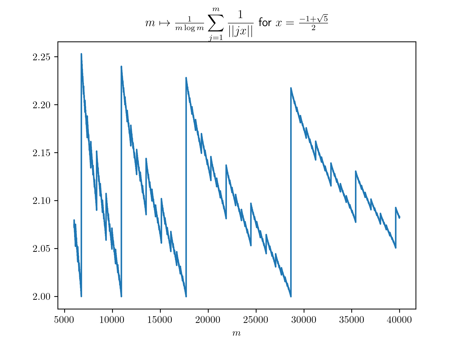
For example, take $x=\frac{-1+\sqrt{5}}{2}$, for which $a_n(x)=1$ for all $n\in \mathbb{N}$, and so in particular $x$ has bounded partial quotients. In Figure 1 we plot $\frac{1}{m\log m}\cdot {\sum }_{j=1}^m\frac{1}{\parallel jx\parallel }$ for $m=5000,\mathrm{\dots },40000$. These computations suggest that there is some constant $C$ for which ${\sum }_{j=1}^m\frac{1}{\parallel jx\parallel }>Cm\log m$ for all $m$. In Theorem 13 we shall prove that for almost all $x\in \mathrm{\Omega }$ there is such a $C(x)$.

Figure 1: $\frac{1}{m\log m}{\sum }_{j=1}^m\frac{1}{\parallel jx\parallel }$ for $x=\frac{-1+\sqrt{5}}{2}$, for $m=5000,\mathrm{\dots },40000$

However, the estimate in Theorem 11 is not true for all $x\in \mathrm{\Omega }$. Define $a\in {\mathbb{N}}^{\mathbb{N}}$ as follows. Let $a_1$ be any element of $\mathbb{N}$. Then inductively, define $a_{n+1}$ to be any element of $\mathbb{N}$ that is $>q_n^{n-1}$. Then for any $n\in \mathbb{N}$, using (11) and $q_{n+1}=a_{n+1}{q}_n+q_{n-1}>a_{n+1}{q}_n$ we get

hence , and then

$$\sum _{j=1}^{q_n}\frac{1}{\parallel jv(a)\parallel }>\frac{1}{\parallel q_{n}v(a)\parallel }>q_n^n.$$

Using $ϵ=1$, it is then straightforward to check that there is no constant $C$ such that ${\sum }_{j=1}^m\frac{1}{\parallel jv(a)\parallel }\le Cm{(\log m)}^2$ for all $m$.

We will need the following lemma [19, p. 324, Lemma 3] to prove a theorem; cf. Khinchin [78, p. 63, Theorem 30].

Lemma 12.

If $\varphi$ is a function defined on the positive integers such that $\varphi \mathit{}\mathrm{(}n\mathrm{)}\mathrm{\ge }\mathrm{1}$ for all $n$ and

then for almost all $x\mathrm{\in }\mathrm{\Omega }$ there are only finitely many $n$ such that $a_n\mathit{}\mathrm{(}x\mathrm{)}\mathrm{\ge }\varphi \mathit{}\mathrm{(}n\mathrm{)}$.

Proof.

For a measurable set $A\subset \mathrm{\Omega }$, define

$$\gamma (A)=\frac{1}{\log 2}{\int }_A\frac{1}{1+x}𝑑\mu (x),$$

in other words $d\gamma (x)=\frac{1}{(1+x)\log 2}d\mu (x)$. Thus for a measurable set $A\subset \mathrm{\Omega }$ we have

$$\gamma (A)\le \frac{1}{\log 2}{\int }_A𝑑x=\frac{1}{\log 2}\mu (A)$$

and

$$\gamma (A)\ge \frac{1}{\log 2}{\int }_A\frac{1}{2}𝑑x=\frac{1}{2\log 2}\mu (A).$$

We will use that $\gamma$ is an invariant measure for the Gauss transformation $T:\mathrm{\Omega }\to \mathrm{\Omega }$ [44, p. 77, Lemma 3.5], i.e., if $A\subset \mathrm{\Omega }$ is a measurable set then

$$(T_{*}\gamma )(A)=\gamma (T^{-1}(A))=\gamma (A).$$

Let $A_n=\{x\in \mathrm{\Omega }:a_n(x)\ge \varphi (n)\}$, $n\ge 1$. As

$$a_n(x)=\left[\frac{1}{T^{n-1}(x)}\right],$$

we have

$A_n$ $\subset$ $\mathrm{\{}x\in \mathrm{\Omega }:{\displaystyle \frac{1}{T^{n-1}(x)}}>\varphi (n)\}$

$=$

$=$ ${(T^{n-1})}^{-1}\left([0,{\displaystyle \frac{1}{\varphi (n)}})\setminus \mathbb{Q}\right).$

Hence

$\mu (A_n)$ $\le$ $\mu \left({(T^{n-1})}^{-1}\left([0,{\displaystyle \frac{1}{\varphi (n)}})\setminus \mathbb{Q}\right)\right)$

$\le$ $2\log 2\cdot \gamma \left({(T^{n-1})}^{-1}\left([0,{\displaystyle \frac{1}{\varphi (n)}})\setminus \mathbb{Q}\right)\right)$

$=$ $2\log 2\cdot \gamma \left([0,{\displaystyle \frac{1}{\varphi (n)}})\setminus \mathbb{Q}\right)$

$\le$ $2\log 2\cdot {\displaystyle \frac{1}{\log 2}}\cdot \mu \left([0,{\displaystyle \frac{1}{\varphi (n)}})\setminus \mathbb{Q}\right)$

$=$ ${\displaystyle \frac{2}{\varphi (n)}}.$

It follows that

and thus by the Borel-Cantelli lemma [19, p. 59, Theorem 4.3] we have

$$\mu (\underset{n\to \mathrm{\infty }}{lim\; sup}{A}_n)=0.$$

∎

Let $\lambda$ be Lebesgue measure on $I=[0,1]$, let $d\gamma (x)=\frac{1}{(1+x)\log 2}d\lambda (x)$, and let $T:I\to I$ be the Gauss transformation, $T(x)=x^{-1}-{[x]}^{-1}$ for $x>0$ and $T(0)=0$, for which $T_{*}\gamma =\gamma$ [44, p. 77, Lemma 3.5]. Suppose that $\nu$ is a Borel probability measure on $[0,1]$ such that the pushforward measure $T_{*}\nu$ is absolutely continuous with respect to $\nu$. For $f\in L^1(\nu )$, define $d{\nu }_f=fd\nu$, and define $P_{\nu }:L^1(\nu )\to L^1(\nu )$ by

$$P_{\nu }f=\frac{d(T_{*}{\nu }_f)}{d\nu },f\in L^1(\nu ).$$

Thus, for $g\in L^{\mathrm{\infty }}(\nu )$, using the change of variables formula,

$${\int }_{I}g\cdot P_{\nu }f𝑑\nu ={\int }_{I}gd(T_{*}{\nu }_f)={\int }_{I}g\circ T𝑑{\nu }_f={\int }_I(g\circ T)\cdot f𝑑\nu ,$$

in particular,

$${\int }_I{P}_{\nu }f𝑑\nu ={\int }_{I}f𝑑\nu .$$

We call $P_{\nu }:L^1(\nu )\to L^1(\nu )$ a Perron-Frobenius operator for $T$. It is a fact that if $f\ge 0$ then $P_{\nu }f\ge 0$ [69, p. 57, Proposition 2.1.1], namely $P_{\nu }\ge 0$. It can be proved that for $f\in L^1(\gamma )$, for almost all $x\in I$ [69, p. 59, Proposition 2.1.2],

$$(P_{\gamma }f)(x)=\sum _{k=1}^{\mathrm{\infty }}\frac{x+1}{(x+k)(x+k+1)}\cdot f\left(\frac{1}{x+k}\right),$$

and for $f\in L^1(\lambda )$, for almost all $x\in I$ [69, p. 60, Corollary 2.1.4],

$$(P_{\lambda }f)(x)=\sum _{k=1}^{\mathrm{\infty }}\frac{1}{{(x+k)}^2}\cdot f\left(\frac{1}{x+k}\right),$$

and with $g(x)=(x+1)f(x)$, for $n\ge 1$ it holds for almost all $x\in I$ that $(P_{\lambda }^{n}f)(x)=\frac{(P_{\gamma }^{n}g)(x)}{x+1}$. Iosifescu and Kraaikamp [69, Chapter 2] give a detailed presentation of Perron-Frobenius operators for the Gauss map. We make the final remark that $P_{\nu }{1}_I=1_I$ is equivalent with ${\int }_I{1}_E𝑑\nu ={\int }_I{1}_{T^{-1}(E)}𝑑\nu$ for all Borel sets $E$ in $I$, i.e. $\nu (E)=\nu (T^{-1}(E))$, which in turn means $T_{*}\nu =\nu$, cf. Markov operators [83, Chapter 5, §5.1, pp. 177-186]. An object similar to Perron-Frobenius operators for the Gauss transformation is the zeta-function for the Gauss transformation, for which see Lagarias [87, p. 58, §3.3].

The following theorem gives a lower bound on the sum ${\sum }_{j=1}^m\frac{1}{\parallel jx\parallel }$, cf. [150, p. 4, Theorem 3.1].

Theorem 13.

For almost all $x\mathrm{\in }\mathrm{\Omega }$ there is some $C\mathrm{>}\mathrm{0}$ such that

$$\sum _{j=1}^m\frac{1}{\parallel jx\parallel }>Cm\log m.$$

Proof.

For all $x\in \mathrm{\Omega }$, if $n\ge 1$ then $q_n\ge 2^{\frac{n-1}{2}}$, by (9). Take $\varphi (n)=2^{\frac{n-2}{2}}$. The series ${\sum }_{n=1}^{\mathrm{\infty }}\frac{1}{\varphi (n)}$ converges, so by Lemma 12, for almost all $x\in \mathrm{\Omega }$ there are only finitely many $n$ such that $a_n\ge \varphi (n)$. That is, for almost all $x\in \mathrm{\Omega }$ there is some $n_0$ such that if $n\ge n_0$ then

Hence, if $n\ge n_0$ then

It follows that for almost all $x\in \mathrm{\Omega }$ there is some $K$ such that

(15)

for all $n\ge 0$.

For such an $x$, let $m$ be a positive integer and let . For $1\le j\le m$ we have by (11),

Therefore for $1\le j\le m$ we have

Let $L=[\frac{m}{q_n}]$, so $L{q}_n\le m$. Then,

${\displaystyle \sum _{j=1}^m}{\displaystyle \frac{1}{\parallel jx\parallel }}$ $>$ ${\displaystyle \sum _{j=1}^m}{\displaystyle \frac{1}{\frac{1}{q_n}+\parallel \frac{j{p}_n}{q_n}\parallel }}$

$\ge$ ${\displaystyle \sum _{l=0}^{L-1}}{\displaystyle \sum _{h=1}^{q_n}}{\displaystyle \frac{1}{\frac{1}{q_n}+\parallel \frac{(l{q}_n+h)p_n}{q_n}\parallel }}$

$=$ $q_n{\displaystyle \sum _{l=0}^{L-1}}{\displaystyle \sum _{h=1}^{q_n}}{\displaystyle \frac{1}{1+q_n\parallel \frac{h{p}_n}{q_n}\parallel }}$

$=$ $L{q}_n{\displaystyle \sum _{h=1}^{q_n}}{\displaystyle \frac{1}{1+q_n\parallel \frac{h{p}_n}{q_n}\parallel }}$

$=$ $L{q}_n{\displaystyle \sum _{k=0}^{q_n-1}}{\displaystyle \frac{1}{1+q_n\cdot \frac{k}{q_n}}}$

$>$ $L{q}_n\log q_n.$

But if $y\ge 1$ then $[y]>\frac{y}{2}$, so $L=[\frac{m}{q_n}]>\frac{m}{2q_n}$. Hence by (15),

$$\sum _{j=1}^m\frac{1}{\parallel jx\parallel }>\frac{m}{2}\log q_n>\frac{m}{2}\log \sqrt{\frac{q_{n+1}}{K}}>\frac{m}{2}\log \sqrt{\frac{m}{K}},$$

and thus there is some $C>0$ such that ${\sum }_{j=1}^m\frac{1}{\parallel jx\parallel }>Cm\log m$ for all $m\ge 1$. ∎

The following is from Kuipers and Niederreiter [85, p. 131, Exercise 3.12].

Theorem 14.

If $x\mathrm{\in }\mathrm{\Omega }$ is of type , then for all $m\mathrm{\ge }\mathrm{1}$ we have

Proof.

Summation by parts is the following identity, which can be easily checked:

$$\sum _{n=1}^N{a}_n(b_{n+1}-b_n)=a_{N+1}{b}_{N+1}-a_1{b}_1-\sum _{n=1}^N{b}_{n+1}(a_{n+1}-a_n).$$

Let $a_j=\frac{1}{j}$, let $s_j={\sum }_{h=1}^j\frac{1}{\parallel hx\parallel }$, let $b_1=0$, and let $b_j=s_{j-1}$ for $j\ge 2$. Doing summation by parts gives

$$\sum _{j=1}^m\frac{1}{j\parallel jx\parallel }=\frac{1}{m+1}{s}_m-\sum _{j=1}^m{s}_j\left(\frac{1}{j+1}-\frac{1}{j}\right)=\frac{1}{m+1}{s}_m+\sum _{j=1}^m{s}_j\frac{1}{j(j+1)}.$$

As $x$ is of type , we can use Theorem 10 to get for each $j\ge 1$. Therefore

${\displaystyle \sum _{j=1}^m}{\displaystyle \frac{1}{j\parallel jx\parallel }}$ ${\displaystyle \frac{1}{m+1}}12m(\psi (m)+\log m)+{\displaystyle \sum _{j=1}^m}{\displaystyle \frac{12(\psi (j)+\log j)}{j+1}}$

$12(\psi (m)+\log m)+12{(\log m)}^2+12{\displaystyle \sum _{j=1}^m}{\displaystyle \frac{\psi (j)}{j+1}}$

$24{(\log m)}^2+12\psi (m)+12{\displaystyle \sum _{j=1}^m}{\displaystyle \frac{\psi (j)}{j+1}}.$

∎

Erdős [45] proves that for almost all $x$,

$$\sum _{j=1}^m\frac{1}{j\parallel jx\parallel }=(1+o(1)){(\log m)}^2.$$

Kruse [84] gives a comprehensive investigation of the sums ${\sum }_{j=1}^m\frac{1}{j^s{\parallel jx\parallel }^t}$, $s,t\ge 0$. The results depend on whether $s$ and $t$ are are less than, equal, or greater than $1$, and on whether . One of the theorems proved by Kruse is the following [84, p. 260, Theorem 7]. If $t>1$ and $0\le s\le t$, and if $ϵ>0$, then for almost all $x$ we have

$$\sum _{j=1}^m\frac{1}{j^s{\parallel jx\parallel }^t}=O\left(m^{t-s}{(\log m)}^{(1+ϵ)t}\right).$$

Haber and Osgood [56, p. 387, Theorem 1] prove that for real $t\ge 1$, $A>1$, $M>0$, $r>0$, there is some $C=C(t,A,M,r)>0$ such that for all $x\in \mathrm{\Omega }$ satisfying , for all positive integers $K$,

We remind ourselves that according to Theorem 4, the elements of $𝒟(r+1)$ are those $x\in \mathrm{\Omega }$ for which there is some $c(x)>0$ such that $q_{n+1}(x)\le C(x)q_n{(x)}^r$ for all $n\ge 1$.

For $x\in \mathbb{Z}+\frac{1}{2}$, define $\{\{x\}\}=\frac{1}{2}$. If $x\notin \mathbb{Z}+\frac{1}{2}$, then there is an integer $m_x$ for which for all integers $n\ne m_x$, and we define $\{\{x\}\}=x-m_x$. Sinai and Ulcigrai [138, p. 96, Proposition 2] prove that if $\alpha$ has bounded partial quotients, then there is some $C(\alpha )$ such that for all $M$,

$$\left|\sum _{m=1}^M\frac{1}{\{\{m\alpha \}\}}\right|\le C(\alpha )M.$$

7 Weyl’s inequality, Vinogradov’s estimate, Farey fractions, and the circle method

Write

$$𝒜=\{(a,q)\in {\mathbb{Z}}^2:\gcd (a,q)=1,q\ge 1\}.$$

We first prove four estimates following Nathanson [107, pp. 104–110, Lemmas 4.8–4.11] that we will use in what follows; cf. Vinogradov [149, p. 26, Chapter I, Lemma 8b].

Lemma 15.

There is some $C$ such that if $\alpha \mathrm{\in }ℝ$, $\mathrm{(}a\mathrm{,}q\mathrm{)}\mathrm{\in }𝒜$, and

$$\left|\alpha -\frac{a}{q}\right|\le \frac{1}{q^2},$$

then

$$\sum _{1\le r\le q/2}\frac{1}{\parallel \alpha r\parallel }\le Cq\log q.$$

Proof.

For $q=1$, ${\sum }_{1\le r\le q/2}\frac{1}{\parallel \alpha r\parallel }=0$. For $q\ge 2$, let $1\le r\le \frac{q}{2}$. As $\gcd (a,q)=1$ and $r\not\equiv 0(modq)$, $ar\not\equiv 0(modq)$. So for ${\mu }_r=\left[\frac{ar}{q}\right]$, there is some $1\le {\sigma }_r\le q-1$ such that $ar={\mu }_{r}q+{\sigma }_r$. Then

$$\parallel \frac{ar}{q}\parallel =\parallel \frac{{\sigma }_r}{q}\parallel \in \{\frac{{\sigma }_r}{q},1-\frac{{\sigma }_r}{q}\}=\{\frac{{\sigma }_r}{q},\frac{q-{\sigma }_r}{q}\}.$$

Put $\frac{s_r}{q}=\parallel \frac{ar}{q}\parallel$, so (i) $s_r={\sigma }_r$ or (ii) $s_r=q-{\sigma }_r$. In case (i), $\frac{s_r}{q}=\frac{ar}{q}-{\mu }_r$. In case (ii), $\frac{s_r}{q}=1-\left(\frac{ar}{q}-{\mu }_r\right)$. In case (i) let ${ϵ}_r=1,m_r={\mu }_r$, and in case (ii) let ${ϵ}_r=-1,m_r={\mu }_r+1$. Thus, whether (i) or (ii) holds we have

$$\frac{s_r}{q}={ϵ}_r\left(\frac{ar}{q}-m_r\right),\frac{s_r}{q}=\parallel \frac{ar}{q}\parallel ,1\le s_r\le \frac{q}{2}.$$

Write

$$\alpha -\frac{a}{q}=\frac{\theta }{q^2},$$

for some real $\theta$, $|\theta |\le 1$. For ${\theta }_r=\frac{2r}{q}\theta$, which satisfies $|{\theta }_r|\le |\theta |\le 1$,

$$\alpha r=\frac{ar}{q}+\frac{r\theta }{q^2}=\frac{ar}{q}+\frac{{\theta }_r}{2q}.$$

Then

$\parallel \alpha r\parallel$ $=\parallel {\displaystyle \frac{ar}{q}}+{\displaystyle \frac{{\theta }_r}{2q}}\parallel$

$=\parallel {ϵ}_r{\displaystyle \frac{s_r}{q}}+m_r+{\displaystyle \frac{{\theta }_r}{2q}}\parallel$

$\ge \parallel {ϵ}_r{\displaystyle \frac{s_r}{q}}+m_r\parallel -\parallel {\displaystyle \frac{{\theta }_r}{2q}}\parallel$

$={\displaystyle \frac{s_r}{q}}-\left|{\displaystyle \frac{{\theta }_r}{2q}}\right|$

$\ge {\displaystyle \frac{s_r}{q}}-{\displaystyle \frac{1}{2q}}.$

Take $1\le r_1,r_2\le \frac{q}{2}$ and suppose that $s_{r_1}=s_{r_2}$. So

$${ϵ}_{r_1}\left(\frac{a{r}_1}{q}-m_{r_1}\right)={ϵ}_{r_2}\left(\frac{a{r}_2}{q}-m_{r_2}\right)$$

hence $a{r}_1\equiv {ϵ}_{r_1}{ϵ}_{r_2}a{r}_2(modq)$. As $\gcd (a,q)=1$, $r_1\equiv {ϵ}_{r_1}{ϵ}_{r_2}{r}_2(modq)$. Because $1\le r_1,r_2\le q$, if $r_1\equiv r_2(modq)$ then $r_1=r_2$ and if $r_1\equiv -r_2(modq)$ then $r_1=\frac{q}{2}$ and $r_2=\frac{q}{2}$, so in any case $r_1=r_2$. Therefore

$$\{\frac{s_r}{q}:1\le r\le \frac{q}{2}\}=\{\frac{s}{q}:1\le s\le \frac{q}{2}\}.$$

Using the two things we have established,

${\displaystyle \sum _{1\le r\le q/2}}{\displaystyle \frac{1}{\parallel \alpha r\parallel }}$ $\le {\displaystyle \sum _{1\le r\le q/2}}{\displaystyle \frac{1}{\frac{s_r}{q}-\frac{1}{2q}}}$

$={\displaystyle \sum _{1\le s\le q/2}}{\displaystyle \frac{1}{\frac{s}{q}-\frac{1}{2q}}}$

$=2q{\displaystyle \sum _{1\le s\le q/2}}{\displaystyle \frac{1}{2s-1}}$

$\le 2q{\displaystyle \sum _{1\le s\le q/2}}{\displaystyle \frac{1}{s}}$

$\le 2q\left(\log {\displaystyle \frac{q}{2}}+\gamma +O(q^{-1})\right)$

$=O(q\log q).$

∎

Lemma 16.

There is some $C$ such that if $\alpha \mathrm{\in }ℝ$, $\mathrm{(}a\mathrm{,}q\mathrm{)}\mathrm{\in }𝒜$, and

$$\left|\alpha -\frac{a}{q}\right|\le \frac{1}{q^2},$$

then for any positive real $V$ and nonnegative integer $h$,

$$\sum _{r=1}^q\min (V,\frac{1}{\parallel \alpha (hq+r)\parallel })\le C(V+q\log q).$$

Proof.

Write

$$\alpha =\frac{a}{q}+\frac{\theta }{q^2},$$

which satisfies $|\theta |\le 1$, and for $1\le r\le q$ define

$${\delta }_r=R(\theta h)+\frac{\theta r}{q},$$

which satisfies . Then

$\alpha (hq+r)$ $=\left({\displaystyle \frac{a}{q}}+{\displaystyle \frac{\theta }{q^2}}\right)(hq+r)$

$=ah+{\displaystyle \frac{ar}{q}}+{\displaystyle \frac{\theta h}{q}}+{\displaystyle \frac{\theta r}{q^2}}$

$=ah+{\displaystyle \frac{ar}{q}}+{\displaystyle \frac{R(\theta h)+[\theta h]}{q}}+{\displaystyle \frac{\theta r}{q^2}}$

$=ah+{\displaystyle \frac{ar+[\theta h]+{\delta }_r}{q}}.$

For $m_r=\left[\frac{ar+[\theta h]+{\delta }_r}{q^2}\right]$,

$$R(\alpha (hq+r))=R\left(\frac{ar+[\theta h]+{\delta }_r}{q}\right)=\frac{ar+[\theta h]+{\delta }_r}{q}-m_r.$$

Suppose that $t\in [0,1-\frac{1}{q}]$ and that $t\le R(\alpha (hq+r))\le t+\frac{1}{q}$. Then

$$qt\le ar+[\theta h]+{\delta }_r-q{m}_r\le qt+1.$$

This implies, as ${\delta }_r\ge -1$,

$$ar-q{m}_r\le qt+1-[\theta h]-{\delta }_r\le qt+1-[\theta h]+1=qt-[\theta h]+2$$

and, as ,

$$ar-q{m}_r\ge qt-[\theta h]-{\delta }_r>qt-[\theta h]-2,$$

so $ar-q{m}_r\in J_t$, writing

$$J_t=(qt-[\theta h]-2,qt-[\theta h]+2].$$

For $1\le r_1,r_2\le q$, if $a{r}_1-q{m}_{r_1}=a{r}_2-q{m}_{r_2}$ then $a{r}_1\equiv a{r}_2(modq)$, and $\gcd (a,q)=1$ implies $r_1\equiv r_2(modq)$; and $1\le r_1,r_2\le q$ so $r_1=r_2$. For $t\in [0,1-\frac{1}{q}]$, four integers belong to $J_t$, hence

$$\{1\le r\le q:ar-q{m}_r\in J_t\}$$

has at most four elements. But

$$\{1\le r\le q:R(\alpha (hq+r))\in [t,t+\frac{1}{q}]\}\subset \{1\le r\le q:ar-q{m}_r\in J_t\}.$$

Now,

whence

$\{1\le r\le q:\parallel \alpha (hq+r)\parallel \in [t,t+{\displaystyle \frac{1}{q}}]\}$ $\subset \{1\le r\le q:ar-q{m}_r\in J_t\}$

$\cup \{1\le r\le q:ar-q{m}_r\in J_{1-\frac{1}{q}-t}\}.$

This shows that if $t\in [0,1-\frac{1}{q}]$ then

$$\{1\le r\le q:\parallel \alpha (hq+r)\parallel \in [t,t+\frac{1}{q}]\}$$

has at most eight elements. For , writing

$$I_k=[\frac{k}{q},\frac{k}{q}+\frac{1}{q}],$$

the set $\{1\le r\le q:\parallel \alpha (hq+r)\parallel \in I_k\}$ has at most eight elements. Therefore

${\displaystyle \sum _{1\le r\le q}}\min (V,{\displaystyle \frac{1}{\parallel \alpha (hq+r)\parallel }})$

$=O(V+q\log q).$

∎

Lemma 17.

There is some $C$ such that if $\alpha \mathrm{\in }ℝ$, $\mathrm{(}a\mathrm{,}q\mathrm{)}\mathrm{\in }𝒜$,

$$\left|\alpha -\frac{a}{q}\right|\le \frac{1}{q^2},$$

$U\ge 1$ is a real number, and $n$ is a positive integer, then

$$\sum _{1\le k\le U}\min (\frac{n}{k},\frac{1}{\parallel \alpha k\parallel })\le C\left(\frac{n}{q}+U+q\right)\log 2qU.$$

Proof.

For $1\le k\le U$ there is some and $1\le r_k\le q$ such that $k=q{h}_k+r_k$, and then

${\displaystyle \sum _{1\le k\le U}}\min ({\displaystyle \frac{n}{k}},{\displaystyle \frac{1}{\parallel \alpha k\parallel }})$

the last inequality by Lemma 15. If then for $h=0$, and if and $1\le r\le q$ then $h\ge \frac{h+1}{2}$ so $hq+r>hq\ge \frac{(h+1)q}{2}$ and hence , whence

Consquently

Lemma 16 with $V=\frac{n}{(h+1)q}$ says

$$\sum _{1\le r\le q}\min (\frac{n}{(h+1)q},\frac{1}{\parallel \alpha (hq+r)\parallel })\le C_2\left(\frac{n}{(h+1)q}+q\log q\right),$$

therefore

${\displaystyle \sum _{1\le k\le U}}\min ({\displaystyle \frac{n}{k}},{\displaystyle \frac{1}{\parallel \alpha k\parallel }})$

$\ll q\log q+{\displaystyle \frac{n}{q}}\log \left({\displaystyle \frac{U}{q}}+1\right)+U\log q$

$\ll U\log 2qU+q\log 2qU+{\displaystyle \frac{n}{q}}\log \left({\displaystyle \frac{U}{q}}+1\right).$

If $U\le q$ then $\frac{U}{q}+1\le 2\le 2qU$, and if $U>q$ then $\frac{U}{q}+1\le U+1\le 2U\le 2qU$, hence

$$\sum _{1\le k\le U}\min (\frac{n}{k},\frac{1}{\parallel \alpha k\parallel })\ll U\log 2qU+q\log 2qU+\frac{n}{q}\log 2qU.$$

∎

Lemma 18.

There is some $C$ such that if $\alpha \mathrm{\in }ℝ$, $\mathrm{(}a\mathrm{,}q\mathrm{)}\mathrm{\in }𝒜$,

$$\left|\alpha -\frac{p}{q}\right|\le \frac{1}{q^2},$$

and $U\mathrm{,}V\mathrm{\ge }\mathrm{1}$ are real numbers, then

$$\sum _{1\le k\le U}\min (V,\frac{1}{\parallel \alpha k\parallel })\le C\left(q+U+V+\frac{UV}{q}\right)\max \{1,\log q\}.$$

Proof.

For $1\le k\le U$ there is some and $1\le r_k\le q$ such that $k=q{h}_k+r_k$, and then, as in the proof of Lemma 17,

${\displaystyle \sum _{1\le k\le U}}\min (V,{\displaystyle \frac{1}{\parallel \alpha k\parallel }})$

Using Lemma 16,

${\displaystyle \sum _{1\le k\le U}}\min (V,{\displaystyle \frac{1}{\parallel \alpha k\parallel }})$

$\ll q\log q+(V+q\log q)\left({\displaystyle \frac{U}{q}}+1\right)$

$\ll q\log q+{\displaystyle \frac{UV}{q}}+V+U\log q.$

∎

Weyl’s inequality [107, p. 114, Theorem 4.3] is the following. For $k\ge 2$ and $ϵ>0$, there is some $C(k,ϵ)$ such that if $\alpha \in ℝ$, $f(x)$ is a real polynomial with highest degree term $\alpha x^k$, $(a,q)\in 𝒜$, and

$$\left|\alpha -\frac{a}{q}\right|\le \frac{1}{q^2},$$

then, writing $S_N(f)={\sum }_{j=1}^N{e}^{2\pi if(j)}$ and $K=2^{k-1}$,

$$|S_N(f)|\le C(k,ϵ)\cdot N^{1+ϵ}{(N^{-1}+q^{-1}+N^{-k}q)}^{\frac{1}{K}}.$$

Weyl’s inequality is proved using Lemma 18.

Montgomery [103, Chapter 3] gives a similar but more streamlined presentation of Weyl’s inequality. Chandrasekharan [29] gives a historical survey of exponential sums.

Vinogradov’s estimate [146, p. 26, Theorem 3.1] states that there is some $C$ such that for $n\ge 2$, $1\le q\le n$, $\gcd (a,q)=1$, and $\left|\alpha -\frac{a}{q}\right|\le q^{-2}$, then

$$|f_n(\alpha )|\le C(n{q}^{-1/2}+n^{4/5}+n^{1/2}{q}^{1/2}){(\log n)}^4,$$ (16)

where $f_n(\alpha )={\sum }_{p\le n}(\log p)e^{2\pi i\alpha p}$; cf. Nathanson [107, p. 220, Theorem 8.5] and Vinogradov [149, p. 131, Chapter IX, Theorem 1]. This is proved using Lemma 17.

Fix $B>0$ and let $P_n={(\log n)}^B$. For $1\le a\le q\le P_n$ and $\gcd (a,q)=1$, let

$${𝔐}_n(q,a)=\{\alpha \in ℝ:\left|\alpha -\frac{a}{q}\right|\le P_n{n}^{-1}\},$$

called a major arc. One checks that there is some $n_B$ such that if $n\ge n_B$, then ${𝔐}_n(q,a)$ and ${𝔐}_n(q^{\prime },a^{\prime })$ are disjoint when $(q,a)\ne (q^{\prime },a^{\prime })$. Let

$${𝔐}_n=\bigcup _{1\le a\le q\le P_n,\gcd (a,q)=1}{𝔐}_n(q,a).$$

The Farey fractions of order $N$ are

$${𝔉}_N=\{\frac{h}{k}:0\le h\le k\le N,\gcd (h,k)=1\}.$$

Cf. the Stern-Brocot tree [55, §4.5]. For early appearances of Farey fractions, see Dickson [35, pp. 155–158, Chapter V]. It is proved by Cauchy that if $h/k$ and $h^{\prime }/k^{\prime }$ are successive elements of ${𝔉}_N$, then $k{h}^{\prime }-h{k}^{\prime }=1$ [59, p. 23, Theorem 28]. Let

$$\varphi (m)=|\{1\le k\le m:\gcd (k,m)=1\}|,$$

the Euler phi function, and write $\mathrm{\Phi }(N)={\sum }_{1\le m\le N}\varphi (m)$. One sees that $|{𝔉}_N|=1+\mathrm{\Phi }(N)$, and it was proved by Mertens [59, p. 268] that

$$\mathrm{\Phi }(N)=\frac{3N^2}{{\pi }^2}+O(N\log N).$$

Let $\lambda$ be Lebesgue measure on $ℝ$. For $n\ge n_B$, because the major arcs are pairwise disjoint,

$\lambda ({𝔐}_n)$ $={\displaystyle \sum _{1\le a\le q\le P_n,\gcd (a,q)=1}}2P_n{n}^{-1}$

$=\left({\displaystyle \sum _{m=1}^{P_n}}\varphi (m)\right)2P_n{n}^{-1}$

$={\displaystyle \frac{6}{{\pi }^2}}{P}_n^3{n}^{-1}+O(P_n^2{n}^{-1}\log P_n).$

Let $I_n=(P_n{n}^{-1},1+P_n{n}^{-1}]$, which for $n>2P_n^2$ contains ${𝔐}_n$. Let

$${𝔪}_n=I_n\setminus {𝔐}_n,$$

called the minor arcs.

With $f_n(\alpha )={\sum }_{p\le n}(\log p)e^{2\pi i\alpha p}$ and

$$R(n)=\sum _{p_1+p_2+p_3=n}(\log p_1)(\log p_2)(\log p_3),$$

we have

$$R(n)={\int }_{I_n}{f}_n{(\alpha )}^3{e}^{-2\pi in\alpha }𝑑\alpha ={\int }_{{𝔐}_n}{f}_n{(\alpha )}^3{e}^{-2\pi in\alpha }𝑑\alpha +{\int }_{{𝔪}_n}{f}_n{(\alpha )}^3{e}^{-2\pi in\alpha }𝑑\alpha .$$

Using (16), it can be proved that for $A>0$ with $B\ge 2A+10$ [146, p. 29, Theorem 3.2],

$${\int }_{{𝔪}_n}{|f_n(\alpha )|}^3𝑑\alpha =O(n^2{(\log n)}^{-A}).$$

Writing

$$𝔖(n)=\left(\prod _{p\nmid n}(1+{(p-1)}^{-3})\right)\prod _{p\mid n}(1-{(p-1)}^{-2}),$$

called the singular series, it is proved, using the Siegel-Walfisz theorem on primes in arithmetic progressions [102, p. 381, Corollary 11.19], that for $A>0$ with $B\ge 2A$ [146, p. 31, Theorem 3.3],

$${\int }_{{𝔐}_n}{f}_n{(\alpha )}^3{e}^{-2\pi in\alpha }𝑑\alpha =\frac{1}{2}{n}^2𝔖(n)+O(n^2{(\log n)}^{-A}).$$

Thus

$$R(n)=\frac{1}{2}{n}^2𝔖(n)+O(n^2{(\log n)}^{-A}),$$

and it follows from this that there is some $n_0$ such that if $n\ge n_0$ is odd then there are primes $p_1,p_2,p_3$ such that $n=p_1+p_2+p_3$.

For integers $a,b$ with $\gcd (a,b)=1$, the Ford circle $C(a,b)$ is the circle in $ℂ$ that touches the line $\mathrm{Im}z=0$ at $z=\frac{a}{b}$ and has radius $\frac{1}{2b^2}$; in other words, $C(a,b)$ is the circle in $ℂ$ with center $\frac{a}{b}+\frac{i}{2b^2}$ and radius $\frac{1}{2b^2}$. It is straightforward to prove that if $C(a,b)$ and $C(c,d)$ are Ford circles, then they are tangent if and only if ${(bc-ad)}^2=1$, and otherwise they are disjoint [4, p. 100, Theorem 5.6]. It is also straightforward to prove [4, p. 101, Theorem 5.7] that if are successive elements of ${𝔉}_N$, then $C(h_1,k_1)$ and $C(h,k)$ touch at

$$\frac{h}{k}-\frac{k_1}{k(k^2+k_1^2)}+\frac{i}{k^2+k_1^2}$$

and $C(h,k)$ and $C(h_2,k_2)$ touch at

$$\frac{h}{k}+\frac{k_2}{k(k^2+k_2^2)}+\frac{i}{k^2+k_2^2}.$$

Bonahon [21, pp. 207 ff., Chapter 8] explains Ford circles in the language of hyperbolic geometry.

We remind ourselves that $|{𝔉}_N|=1+\mathrm{\Phi }(N)=1+{\sum }_{m=1}^N\varphi (m)$ and let be the elements of ${𝔉}_N$. In particular, ${\rho }_{0,N}=0$ and ${\rho }_{\mathrm{\Phi }(N),N}=1$. For ${\rho }_{n,N}=\frac{h_{n,N}}{k_{n,N}}$ with $\gcd (h_{h,N},k_{n,N})=1$, write $C_{n,N}=C(h_{n,N},k_{n,N})$.

Let $A_{0,N}$ be the clockwise arc of $C_{0,N}$ from $i$ to the point at which $C_{0,N}$ and $C_{1,N}$ touch. For , let $A_{n,N}$ be the clockwise arc of $C_{n,N}$ from the point at which $C_{n-1,N}$ and $C_{n,N}$ touch to the point at which $C_{n,N}$ and $C_{n+1,N}$ touch. Finally, let $A_{\mathrm{\Phi }(N),N}$ be the clockwise arc of $C_{\mathrm{\Phi }(N),N}$ from the point at which $C_{\mathrm{\Phi }(N)-1,N}$ and $C_{\mathrm{\Phi }(N),N}$ touch to $i+1$. Let $A_N$ be the composition of the arcs

$$A_{0,N},\mathrm{\dots },A_{\mathrm{\Phi }(N),N},$$ (17)

which is a contour from $i$ to $i+1$.

Write $H=\{\tau \in ℂ:\mathrm{Im}\tau >0\}$. The Dedekind eta function $\eta :H\to ℂ$ is defined by

$$\eta (\tau )=e^{\pi i\tau /12}\prod _{m=1}^{\mathrm{\infty }}(1-e^{2\pi im\tau }).$$

It is straightforward to check that $\eta$ is analytic and that $\eta (\tau )\ne 0$ for all $\tau \in H$ [143, pp. 17–18, §1.44]. For $(h,k)\in 𝒜$, let

$$s(h,k)=\sum _{r=1}^{k-1}\frac{r}{k}\left(\frac{hr}{k}-\left[\frac{hr}{k}\right]-\frac{1}{2}\right)=\sum _{r=1}^{k-1}\frac{r}{k}{P}_1(hr/k),$$

called a Dedekind sum; $P_1$ is the periodic Bernoulli function. Also, for write

$$ϵ(a,b,c,d)=\exp \left(\pi i\left(\frac{a+d}{12c}+s(-d,c)\right)\right).$$

The functional equation for the Dedekind eta function [4, p. 52, Theorem 3.4] is

Let $p(n)$ be the number of ways of writing $n$ as a sum of positive integers where the order does not matter, called the partition function. For example, $4,3+1,2+2,2+1+1,1+1+1+1$ are the partitions of $4$, so $p(4)=5$. Denoting by $D(0,1)$ the open disc with center $0$ and radius $1$, define $F:D(0,1)\to ℂ$ by

$$F(z)=\prod _{m=1}^{\mathrm{\infty }}{(1-z^m)}^{-1}=\sum _{n=0}^{\mathrm{\infty }}p(n)z^n;$$

that the product and the series are equal was found by Euler. $F$ is analytic. On the one hand, $p(n)=\frac{F^{(n)}(0)}{n!}$, and on the other hand, by Cauchy’s integral formula [143, p. 82, Theorem 2.41], if $C$ is a circle with center $0$ and radius then

$$F^{(n)}(0)=\frac{n!}{2\pi i}{\int }_C\frac{F(z)}{z^{n+1}}𝑑z.$$

Taking $C$ to be the circle with center $0$ and radius $e^{-2\pi }$ and doing the change of variable $z=e^{2\pi i\tau }$,

$p(n)$ $={\displaystyle \frac{1}{2\pi i}}{\displaystyle {\int }_i^{i+1}}{\displaystyle \frac{F(e^{2\pi i\tau })}{e^{2\pi i(n+1)\tau }}}\cdot 2\pi i{e}^{2\pi i\tau }𝑑\tau$

$={\displaystyle {\int }_i^{i+1}}F(e^{2\pi i\tau })e^{-2\pi in\tau }𝑑\tau$

$={\displaystyle {\int }_{A_N}}F(e^{2\pi i\tau })e^{-2\pi in\tau }𝑑\tau ,$

where we remind ourselves that $A_N$ is the contour (17) from $i$ to $i+1$. Using this and the functional equation for the Dedekind eta function, Rademacher [4, p. 104, Theorem 5.10] proves that for $n\ge 1$,

$$p(n)=\frac{1}{\pi \sqrt{2}}\sum _{k=1}^{\mathrm{\infty }}{A}_k(n)k^{1/2}\frac{d}{dn}\frac{\sinh \left(\pi \sqrt{\frac{2}{3}}\cdot \frac{1}{k}\sqrt{n-\frac{1}{24}}\right)}{\sqrt{n-\frac{1}{24}}},$$

for .

We make a final remark about the Farey fractions. Writing the elements of ${𝔉}_N$ as , let ${\eta }_{n,N}={\rho }_{n,N}-\frac{n}{\mathrm{\Phi }(N)}$ for $1\le n\le N$. For example, $\mathrm{\Phi }(5)=10$ and

$$\{{\rho }_{1,5},\mathrm{\dots },{\rho }_{10,5}\}=\{\frac{1}{5},\frac{1}{4},\frac{1}{3},\frac{2}{5},\frac{1}{2},\frac{3}{5},\frac{2}{3},\frac{3}{4},\frac{4}{5},1\},$$

and

$$\{{\eta }_{1,5},\mathrm{\dots },{\eta }_{10,5}\}=\{\frac{1}{10},\frac{1}{20},\frac{1}{30},0,0,0,-\frac{1}{30},-\frac{1}{20},-\frac{1}{10},0\}.$$

Landau [91], following work of Franel, proves that the Riemann hypothesis is true if and only if for every $ϵ>0$,

$$\sum _{n=1}^{\mathrm{\Phi }(N)}|{\eta }_{n,N}|=O(N^{\frac{1}{2}+ϵ}).$$

For example, for $N=5$, the left-hand side is $\frac{11}{30}$. See Narkiewicz [106, p. 40, §2.2.3].

8 Discrepancy and exponential sums

Discrepancy and Diophantine approximation are covered by Kuipers and Niederreiter [85, Chapters 1–2 ] and by Drmota and Tichy [41, §§1.1–1.4], especially [41, pp. 48–66, §1.4.1].

Let $\omega =(x_n)$, $n\ge 1$, be a sequence of real numbers, and let $E\subset [0,1)$. For a positive integer $N$, let $A(E;N;\omega )$ be the number of $x_n$, $1\le n\le N$, such that $R(x_n)\in E$. We say that the sequence $\omega$ is uniformly distributed modulo $\mathrm{1}$ if we have for all $a$ and $b$ with that

$$\underset{N\to \mathrm{\infty }}{lim}\frac{A([a,b);N;\omega )}{N}=b-a.$$

It can be shown [85, p. 3, Corollary 1.1] that a sequence $x_n$ is uniformly distributed modulo $1$ if and only if for every Riemann integrable function $f:[0,1]\to ℝ$ we have

$$\underset{N\to \mathrm{\infty }}{lim}\frac{1}{N}\sum _{n=1}^{N}f(R(x_n))={\int }_0^{1}f(t)𝑑t.$$ (18)

Thus, if a sequence is uniformly distributed then the integral of any Riemann integrable function on $[0,1]$ can be approximated by sampling according to this sequence. This approximation can be quantified using the notion of discrepancy.

It can be proved [85, p. 7, Theorem 2.1] that a sequence $x_n$ is uniformly distributed modulo $1$ if and only if for all nonzero integers $h$ we have

$$\underset{N\to \mathrm{\infty }}{lim}\frac{1}{N}\sum _{n=1}^N{e}^{2\pi ih{x}_n}=0;$$

this is called Weyl’s criterion. But if $x\in \mathrm{\Omega }$, then

$$\left|\sum _{n=1}^N{e}^{2\pi ihnx}\right|=\left|\frac{1-e^{2\pi ihNx}}{1-e^{2\pi ihx}}\right|\le \frac{2}{|1-e^{2\pi ihx}|}=\frac{1}{|\sin \pi hx|}.$$ (19)

We thus obtain the following theorem.

Theorem 19.

If $x\mathrm{\in }\mathrm{\Omega }$ then the sequence $n\mathit{}x$ is uniformly distributed modulo $\mathrm{1}$.

The discrepancy of a sequence $\omega$ is defined, for $N$ a positive integer, by

One proves that the sequence $\omega$ is uniformly distributed modulo $1$ if and only if $D_N(\omega )\to 0$ as $N\to \mathrm{\infty }$ [85, p. 89, Theorem 1.1].

For $f:[0,1]\to ℝ$, let $V(f)$ denote the total variation of $f$. Koksma’s inequality [85, p. 143, Theorem 5.1] states that for any sequence $\omega =(x_n)$, for any $f:[0,1]\to ℝ$ of bounded variation, and for any positive integer $N$, we have

$$\left|\frac{1}{N}\sum _{n=1}^{N}f(R(x_n))-{\int }_0^{1}f(t)𝑑t\right|\le V(f)D_N(\omega ).$$ (20)

Following Kuipers and Niederreiter [85, p. 122, Lemma 3.2], we can bound the discrepancy of the sequence $nx$ in terms of the sum on the left-hand side of Theorem 14

Lemma 20.

There is some $C\mathrm{>}\mathrm{0}$ such that for all $x\mathrm{\in }\mathrm{\Omega }$, $\omega \mathrm{=}\mathrm{(}n\mathit{}x\mathrm{)}$, and for all positive integers $m$ we have

Proof.

We shall use the following inequality, which lets us bound the discrepancy of a sequence in terms of exponential sums formed from the elements of the sequence. The Erdős-Turán theorem [85, p. 114, Eq. 2.42] states that there is some constant $C>0$ such that for any sequence $\omega =(x_n)$ of real numbers, any positive integer $N$, and any positive integer $m$ we have

$$D_N(\omega )\le C\left(\frac{1}{m}+\sum _{j=1}^m\frac{1}{j}\left|\frac{1}{N}\sum _{n=1}^N{e}^{2\pi ij{x}_n}\right|\right).$$ (21)

Take $x_n=nx$. For each $j\ge 1$, by (19) we have

$$\left|\sum _{n=1}^N{e}^{2\pi ijnx}\right|\le \frac{1}{|\sin \pi jx|}=\frac{1}{\sin (\pi \parallel jx\parallel )}.$$

But $\sin t\ge \frac{2}{\pi }t$ for $0\le t\le \frac{\pi }{2}$, so

Using this in (21) gives us

which is the claim. ∎

It follows from Theorem 14 and Lemma 20 (taking $m=N$) that if $x$ is of type then

$$D_N(\omega )=O\left(\frac{{(\log N)}^{2+ϵ}}{N}\right).$$ (22)

Lemma 8 tells us that for almost all $x\in \mathrm{\Omega }$ there is some $K>0$ such that $x$ is of type , so for almost all $x\in \mathrm{\Omega }$, the bound (22) is true. It likewise follows that if $x$ has bounded partial quotients then

$$D_N(\omega )=O\left(\frac{{(\log N)}^2}{N}\right).$$ (23)

In fact, it can be proved that if $x\in {ℬ}_K$ then, for $g=\frac{1+\sqrt{5}}{2}$ [85, p. 125, Theorem 3.4],

$$D_N(\omega )\le 3N^{-1}+\left(\frac{1}{\log g}+\frac{K}{\log (K+1)}\right)N^{-1}\log N.$$

We use the above bounds in the proof of the following theorem.

Theorem 21.

Let $ϵ\mathrm{>}\mathrm{0}$. For almost all $x$ we have

$$\sum _{n=1}^N\parallel nx\parallel =\frac{N}{4}+O({(\log N)}^{2+ϵ}),$$

while if $x$ has bounded partial quotients then

$$\sum _{n=1}^N\parallel nx\parallel =\frac{N}{4}+O({(\log N)}^2).$$

Proof.

Let $f(t)=\parallel t\parallel$. Then $V(f)=1$ and ${\int }_0^{1}f(t)𝑑t=\frac{1}{4}$, so we get from Koksma’s inequality (20) that

$$|\frac{1}{N}\sum _{n=1}^N\parallel nx\parallel -\frac{1}{4}|\le D_N(\omega ),$$

thus

$$\sum _{n=1}^N\parallel nx\parallel =\frac{N}{4}+O(N{D}_N(\omega )).$$

The claims then follow respectively from (22) and (23). ∎

Like we mentioned at the beginning of §6, because $|\sin (\pi x)|=\sin (\pi \parallel x\parallel )\le \pi \parallel x\parallel$ and $|\sin (\pi x)|=\sin (\pi \parallel x\parallel )\ge \frac{2}{\pi }\cdot \pi \parallel x\parallel =2\parallel x\parallel$, we have

$$2\sum _{n=1}^N\parallel nx\parallel \le \sum _{n=1}^N|\sin (\pi nx)|\le \pi \sum _{n=1}^N\parallel nx\parallel .$$

Thus Theorem 21 also gives estimates for ${\sum }_{n=1}^N|\sin (\pi nx)|$.

We can investigate the sum ${\sum }_{n=1}^{N}R(nx)$ rather than ${\sum }_{n=1}^N\parallel nx\parallel$; see Lang [92, p. 37, Theorem 1], who proves that for almost all $x\in \mathrm{\Omega }$,

$$\sum _{n=1}^{N}R(nx)=\frac{N}{2}+O({(\log N)}^{2+ϵ}).$$

For $x\in \mathrm{\Omega }$, let $q_n=q_n(x)$, the denominator of the $n$th convergent of the continued fraction expansion of $x$, and let $a_n=a_n(x)$, the $n$th partial quotient of the continued fraction expansion of $x$. For $m\ge 1$, one can prove [18, p. 211, Proposition 1] that $m$ can be written in one and only one way in the form

$$m=\sum _{k=1}^{\mathrm{\infty }}{z}_k{q}_{k-1}=\sum _{k=1}^t{z}_k{q}_{k-1},$$ (24)

where (i) $0\le z_1\le a_1-1$, (ii) $0\le z_k\le a_k$ for $k\ge 2$, (iii) for $k\ge 1$, if $z_{k+1}=a_{k+1}$ then $z_k=0$, and (iv) $z_t\ne 0$ and $z_k=0$ for $k>t$. The expression (24) is called the Ostrowski expansion of $m$. We emphasize that this expansion depends on $x$. Berthé [18] surveys applications of this numeration system in combinatorics. For $n\ge 0$, define $d_{2n}=q_{2n}x-p_{2n}$ and $d_{2n+1}=p_{2n+1}-q_{2n+1}x$. Brown and Shiue [24, p. 184, Theorem 1] prove that for $x\in \mathrm{\Omega }$,

$$\sum _{k=1}^m\left(R(kx)-\frac{1}{2}\right)=\sum _{k=1}^t{(-1)}^k{z}_k\left(\frac{1}{2}-d_{k-1}\left(m_{k-1}+\frac{1}{2}{z}_k{q}_{k-1}+\frac{1}{2}\right)\right),$$ (25)

where $m_0=0$ and if $k\ge 1$ then $m_k={\sum }_{j=1}^k{z}_j{q}_{j-1}$. If $k\ge 0$, then by (11) we have . For $k\ge 1$, using the fact that $q_k\ge m_k+1$ (for the same reason that if the highest power of $2$ appearing in a number’s binary expansion is $2^{k-1}$, then the number is $\le 2^k-1$),

$m_{k-1}+{\displaystyle \frac{1}{2}}{z}_k{q}_{k-1}+{\displaystyle \frac{1}{2}}$ $=$ $m_k-{\displaystyle \frac{1}{2}}{z}_k{q}_{k-1}+{\displaystyle \frac{1}{2}}$

$\le$ $q_k-1-{\displaystyle \frac{1}{2}}{z}_k{q}_{k-1}+{\displaystyle \frac{1}{2}}$

$=$ $q_k-{\displaystyle \frac{1}{2}}-{\displaystyle \frac{1}{2}}{z}_k{q}_{k-1}$

$q_k.$

Using (25), this inequality, and the inequality , we obtain

$\left|{\displaystyle \sum _{k=1}^m}\left(R(kx)-{\displaystyle \frac{1}{2}}\right)\right|$ $\le$ ${\displaystyle \sum _{k=1}^t}{z}_k\left|{\displaystyle \frac{1}{2}}-d_{k-1}\left(m_{k-1}+{\displaystyle \frac{1}{2}}{z}_k{q}_{k-1}+{\displaystyle \frac{1}{2}}\right)\right|$

${\displaystyle \frac{1}{2}}{\displaystyle \sum _{k=1}^t}{z}_k$

${\displaystyle \frac{1}{2}}{\displaystyle \sum _{k=1}^t}{a}_k.$

If the continued fraction expansion of $x$ has bounded partial quotients, say $a_k\le K$ for all $k$, we obtain from the above that

It can be proved [24, p. 185, Fact 2] that . Thus, if $a_k\le K$ for all $k$, then for $m\ge 1$,

This is Lerch’s claim stated in §3. For example, if $x=\frac{-1+\sqrt{5}}{2}\in \mathrm{\Omega }$ then $a_k(x)=1$ for all $k\ge 1$. We compute that

$$\sum _{k=1}^{1000000}\left(R(kx)-\frac{1}{2}\right)=0.941799\mathrm{\dots };$$

on the other hand, we compute that

$$\sum _{k=1}^{1000000}\left(R(k\pi )-\frac{1}{2}\right)=19.223414\mathrm{\dots }.$$

Brown and Shiue [24, p. 185, Fact 1] use (25) to obtain the result of Sierpinski stated in §3 that for all $x\in \mathrm{\Omega }$,

$$\sum _{k=1}^{m}R(kx)=\frac{m}{2}+o(m).$$

They also prove [24, p. 188, Theorem 4] that for $A>0$, there exists some $d_A>0$ such that for $x\in \mathrm{\Omega }$, if there are infinitely many $t$ such that ${\sum }_{k=1}^t{a}_k\le At$ (which happens in particular if $x$ has bounded partial quotients), then there are infinitely many $m$ such that

$$\sum _{k=1}^m\left(R(kx)-\frac{1}{2}\right)>d_A\log m,$$

and there are infinitely many $m$ such that

It can be shown [92, p. 44, Theorem 4] that if $k$ is a positive integer and $ϵ>0$, then for almost all $x$ we have

$$\left|\sum _{n=1}^N{e}^{2\pi i{n}^{k}x}\right|=O\left(N^{\frac{1}{2}+ϵ}\right).$$

Lang attributes this result to Vinogradov. But it is not so easy to obtain a bound on this exponential sum for specific $x$. For $k=2$, one can prove [92, p. 45, Lemma] that for any $x\in \mathrm{\Omega }$,

cf. Steele [142, Problem 14.2]. By (14) this gives us

If $x$ has bounded partial quotients, it follows from Theorem 11 that

$$\left|\sum _{n=1}^N{e}^{2\pi i{n}^{2}x}\right|=O\left(N^{1/2}{(\log N)}^{1/2}\right).$$

Hardy and Littlewood [57, p. 28, Theorem B5] prove that if $x\in \mathrm{\Omega }$ is an algebraic number, then there is some such that ${\sum }_{n=1}^{N}R(nx)=\frac{N}{2}+O(N^{\alpha (x)})$. Pillai [115] gives a different proof of this.

Theorem 22 (Hardy and Littlewood, Pillai).

For $\tau \mathrm{>}\mathrm{2}$, if $x\mathrm{\in }𝒟\mathit{}\mathrm{(}\tau \mathrm{)}$ then for $\alpha \mathrm{=}\frac{\tau \mathrm{-}\mathrm{2}}{\tau \mathrm{-}\mathrm{1}}$,

$$\sum _{n=1}^{N}R(nx)=\frac{N}{2}+O(N^{\alpha }).$$

Pillai [114] proves other identities and inequalities for ${\sum }_{n=1}^{N}R(nx)$, some for all $x\in \mathrm{\Omega }$ and some for all algebraic $x\in \mathrm{\Omega }$.

For $\omega =(x_n)$, $n\ge 1$ and for $E\subset [0,1)$, we remind ourselves that $A(E;M;\omega )$ denotes the number of $x_n$, $1\le n\le M$, such that $R(x_n)\in E$. Define for $M\ge 1$,

It is straightforward to prove that $D_M^{*}\le D_M\le 2D_M^{*}$ [85, p. 91, Theorem 1.3]. For $N\ge 1$ write $r=\log N$. Let ${ϵ}_0>0$ and let $N^{1/2}\le \tau \le N\exp (-r^{{ϵ}_0})$. Suppose that $\alpha \in ℝ$ and

$$\alpha =\frac{a}{q}+\frac{\theta }{q\tau },\gcd (a,q)=1,\exp (r^{{ϵ}_0})\le q\le \tau ,|\theta |\le 1.$$

For denote by $H_{\beta }(N)$ the number of primes $p\le N$ such that $R(\alpha p)\le \beta$. Vinogradov [149, p. 177, Chapter XI, Theorem] proves that for $ϵ>0$,

$$H_{\beta }(N)=\beta \pi (N)+O(N{(q^{-1}+q{N}^{-1})}^{\frac{1}{2}-ϵ}+N^{\frac{4}{5}+ϵ}),N\to \mathrm{\infty }.$$

Let $\omega =(p_n\alpha )$, $n\ge 1$, where $p_n$ is the $n$th prime. Using Vinogradov’s estimate, one proves that for $\alpha \in ℝ\setminus \mathbb{Q}$, $D_N^{*}(\omega )\to 0$ as $N\to \mathrm{\infty }$, which implies that the sequence $(p_n\alpha )$ is uniformly distributed modulo $1$. A clean proof of this is given by Pollicott [116, p. 200, Theorem 1], and this is also proved by Vaaler [145] using a Tauberian theorem. See also the early survey by Hua [68, pp. 98–99, §38].

Defining $S_{\alpha }(n)={\sum }_{k=1}^n\left(R(k\alpha )-\frac{1}{2}\right)$, Beck [11, p. 14, Theorem 3.1] proves that there is some $c>0$ such that for every $\lambda \in ℝ$,

$$\frac{1}{N}\left|\{1\le n\le N:\frac{S_{\sqrt{2}}(n)}{c\sqrt{\log n}}\le \lambda \}\right|\to \frac{1}{\sqrt{2\pi }}{\int }_{-\mathrm{\infty }}^{\lambda }\exp \left(-\frac{u^2}{2}\right)𝑑u$$

as $N\to \mathrm{\infty }$. Beck [12, p. 20, Theorem 1.2] further proves that if $\alpha$ is a quadratic irrational, there are $C_1=C_1(\alpha )\in ℝ$ and $C_2=C_2(\alpha )\in {ℝ}_{>0}$ such that for $A,B\in ℝ$, ,

Beck and Chen [10]

9 Dirichlet series

The result of de la Vallée-Poussin [34] stated in §3 implies that there is no $s$ such that for all irrational $x$ the Dirichlet series ${\sum }_{n=1}^{\mathrm{\infty }}\frac{n^{-s}}{|\sin n\pi x|}$ converges. It follows from this fact that there is no $s$ such that for all irrational $x$ the Dirichlet series ${\sum }_{n=1}^{\mathrm{\infty }}\frac{n^{-s}}{\parallel nx\parallel }$ converges.

Lerch [97] in 1904 gives some statements without proof about the series

$$\sum _{\nu =1}^{\mathrm{\infty }}\frac{\cot \nu \omega \pi }{{(2\nu \pi )}^{2m+1}}.$$

He states that if $\omega$ is a real algebraic number that does not belong to $\mathbb{Q}$, then for sufficiently large $m$ this series converges, and states, for example, that with $\omega =\frac{1+\sqrt{5}}{2}$,

$$\sqrt{5}\sum _{\nu =1}^{\mathrm{\infty }}\frac{\cot \nu \omega \pi }{{(2\nu \pi )}^7}=-\frac{8}{10!}.$$

Writing $c_r(\theta )={\sum }_{n=1}^{\mathrm{\infty }}\frac{\cot (\pi n\theta )}{n^{2r-1}}$, Berndt [17, p. 135, Theorem 5.1] proves that if $\theta$ is a real algebraic number of degree $d$ and (to say that $d>1$ is to say that $\theta$ is irrational), then $c_r(\theta )$ converges.

For a Dirichlet series ${\sum }_{n=1}^{\mathrm{\infty }}{a}_n{n}^{-s}$, one can show [143, pp. 289–290, §9.11] that if the series is convergent at $s={\sigma }_0+i{t}_0$, then for $\sigma >{\sigma }_0$ and any $t$ the series is convergent at $s=\sigma +it$. It follows that there is some ${\sigma }_0\in [-\mathrm{\infty },\mathrm{\infty }]$ such if then the series diverges at $s=\sigma +it$, and if $\sigma >{\sigma }_0$ then the series converges at $s=\sigma +it$. We call ${\sigma }_0$ the abscissa of convergence of the Dirichlet series. If each $a_n$ is a nonnegative real number, then the function

$$F(s)=\sum _{n=1}^{\mathrm{\infty }}{a}_n{n}^{-s},\mathrm{Re}s>{\sigma }_0,$$

cannot be analytically continued to any domain that includes $s={\sigma }_0$ [67, p. 101, Proposition 18].

Let $a_n$ be a sequence of complex numbers. It can be shown [143, pp. 292–293, §9.14] that if $s_n=a_1+\mathrm{\dots }+a_n$ and the sequence $s_n$ diverges, then the abscissa of convergence of the Dirichlet series ${\sum }_{n=1}^{\mathrm{\infty }}{a}_n{n}^{-s}$ is given by

$${\sigma }_0=\underset{n\to \mathrm{\infty }}{lim\; sup}\frac{\log |s_n|}{\log n}.$$

By Theorem 11 and Theorem 13 (taking, say, $ϵ=1$), for almost all $x\in \mathrm{\Omega }$ there are $C_1,C_2$ such that for all positive integers $n$ we have

Thus, if $a_n=\frac{1}{\parallel nx\parallel }$, then

and hence

$$\underset{n\to \mathrm{\infty }}{lim}\frac{\log s_n}{\log n}=1.$$

It follows that for almost all $x\in \mathrm{\Omega }$ the abscissa of convergence of the Dirichlet series ${\sum }_{n=1}^{\mathrm{\infty }}\frac{1}{\parallel nx\parallel }{n}^{-s}$ is ${\sigma }_0=1$.

Likewise, by Theorem 21 (taking $ϵ=1$), we get for almost all $x\in \mathrm{\Omega }$ that ${\sum }_{j=1}^n\parallel jx\parallel =\frac{n}{4}+O\left({(\log n)}^3\right)$. We can then check that ${lim}_{n\to \mathrm{\infty }}\frac{\log s_n}{\log n}=1$, and hence that the abscissa of convergence of the Dirichlet series ${\sum }_{n=1}^{\mathrm{\infty }}\parallel nx\parallel n^{-s}$ is ${\sigma }_0=1$.

A 1953 result of Mahler [48, pp. 107–108] implies that if $\alpha \in ℝ$ is an algebraic number of degree $d$, then, for $m=[20\cdot 2^{\frac{5(d-1)}{2}}]$, the Dirichlet series

$$\sum _{n=1}^{\mathrm{\infty }}\frac{n^{-s}}{\sin n\alpha }$$

has abscissa of convergence ${\sigma }_0\le d(m+1)\log (m+1)$, and the power series

$$\sum _{n=1}^{\mathrm{\infty }}\frac{z^n}{\sin n\alpha }$$

has radius of convergence 1.

Rivoal [126] presents later work on similar Dirichlet series. See also Queffélec and Queffélec [120]. Lalín, Rodrigue and Rogers [88] prove results about Dirichlet series of the form ${\sum }_{n=1}^{\mathrm{\infty }}\frac{n^{-s}}{\cos (n\pi z)}$. Duke and Imamoḡlu [42] review Hardy and Littlewood’s work on estimating lattice points in triangles, and prove results about lattice points in cones.

For $\theta \in \mathrm{\Omega }$, write

$$R_{r,\theta }(\zeta ,m)=\sum _{n=0}^m\frac{1}{r!}{P}_r(\zeta +n\theta ),$$

where $P_r$ is a periodic Bernoulli function. Spencer [141] proves that for any $ϵ>0$ and almost all $\theta \in \mathrm{\Omega }$,

$$R_{1,\theta }(\zeta ,m)=O\left({(\log m)}^{1+ϵ}\right).$$

Another result Spencer proves in this paper is that if $q_n(\theta )=O(q_{n-1}^h)$, then $R_{r,\theta }(\zeta ,m)=O(m^{1-\frac{r}{h}})$ for . Schoißengeier [132] gives an explicit formula for ${\sum }_{k=0}^{N-1}{P}_2(k\alpha )$.

10 Power series

For a power series $\sum a_n{z}^n$ with radius of convergence $0\le R\le \mathrm{\infty }$, the Cauchy-Hadamard formula [124, p. 111, Chapter 4, §1] states

$$R=\frac{1}{{lim\; sup}_{n\to \mathrm{\infty }}{|a_n|}^{1/n}}=\underset{n\to \mathrm{\infty }}{lim\; inf}{|a_n|}^{-1/n}.$$ (26)

The radius of convergence $R$ is equal to the supremum of those $t\ge 0$ for which $|a_n|t^n$ is a bounded sequence.

Lemma 23.

If $x\mathrm{\in }\mathrm{\Omega }$, then the power series

$$\sum _{n=1}^{\mathrm{\infty }}\frac{z^n}{\parallel nx\parallel }$$

and

$$\sum _{n=1}^{\mathrm{\infty }}\frac{z^n}{|\sin \pi nx|},$$

have the same radius of convergence.

Proof.

The radii of convergence of these power series are respectively

$$\underset{n\to \mathrm{\infty }}{lim\; inf}{\parallel nx\parallel }^{1/n}\mathit{\hspace{1em}}\text{and}\mathit{\hspace{1em}}\underset{n\to \mathrm{\infty }}{lim\; inf}{|\sin (\pi nx)|}^{1/n}.$$

On the one hand,

$$|\sin (\pi nx)|=\sin (\pi \parallel nx\parallel )\le \pi \parallel nx\parallel$$

Therefore, since ${lim}_{n\to \mathrm{\infty }}{\pi }^{1/n}=1$,

$$\underset{n\to \mathrm{\infty }}{lim\; inf}{|\sin (\pi nx)|}^{1/n}\le \underset{n\to \mathrm{\infty }}{lim\; inf}{\left(\pi \parallel nx\parallel \right)}^{1/n}=\underset{n\to \mathrm{\infty }}{lim\; inf}{\parallel nx\parallel }^{1/n}$$

On the other hand, since $\sin t\ge \frac{2}{\pi }t$ for $t\ge 0$,

$$|\sin (\pi nx)|=\sin (\pi \parallel nx\parallel )\ge \frac{2}{\pi }\pi \parallel nx\parallel =2\parallel nx\parallel .$$

Therefore, using ${lim}_{n\to \mathrm{\infty }}{2}^{1/n}=1$, we have

$$\underset{n\to \mathrm{\infty }}{lim\; inf}{|\sin (\pi nx)|}^{1/n}\ge \underset{n\to \mathrm{\infty }}{lim\; inf}{\left(2\parallel nx\parallel \right)}^{1/n}=\underset{n\to \mathrm{\infty }}{lim\; inf}{\parallel nx\parallel }^{1/n},$$

showing that the two power series have the same radius of convergence. ∎

We show in the following theorem that for almost all $x$, the power series ${\sum }_{n=1}^{\mathrm{\infty }}\frac{z^n}{\parallel nx\parallel }$ has radius of convergence $1$.

Theorem 24.

For almost all $x\mathrm{\in }\mathrm{\Omega }$, the power series

$$\sum _{n=1}^{\mathrm{\infty }}\frac{z^n}{\parallel nx\parallel }$$ (27)

has radius of convergence $\mathrm{1}$.

Proof.

For $x\in \mathrm{\Omega }$, let $R_x$ be the radius of convergence of the power series (27). We have , so $\frac{1}{\parallel nx\parallel }>2$. Therefore ${\sum }_{n=1}^N\frac{1}{\parallel nx\parallel }\to \mathrm{\infty }$ as $N\to \mathrm{\infty }$, and so the power series (27) diverges at $z=1$. Therefore $R_x\le 1$ for all $x\in \mathrm{\Omega }$.

We shall use Lemma 7 to get a lower bound on $R_x$ that holds for almost all $x\in \mathrm{\Omega }$. Let , let , and let $B_m$ be those $x\in \mathrm{\Omega }$ such that infinitely often. If $x\in A_m$, then , and this implies that there are infinitely many $n$ such that , so $x\in B_m$, i.e. $A_m\subset B_m$. But let $f_m(n)={\left(1-\frac{1}{m}\right)}^n$. Then ${\sum }_{n=1}^{\mathrm{\infty }}{f}_m(n)$ converges, since , so, by Lemma 7, for almost all $x\in \mathrm{\Omega }$ there are only finitely many $n$ such that . Thus $\mu (B_m)=0$. Hence $\mu (A_m)=0$, and since $A={\bigcup }_{m=2}^{\mathrm{\infty }}{A}_m$ we get that

$$\mu (A)\le \sum _{m=2}^{\mathrm{\infty }}\mu (A_m)=0,$$

that is, $R_x\ge 1$ for almost all $x\in \mathrm{\Omega }$. In conclusion, $R_x=1$ for almost all $x\in \mathrm{\Omega }$. ∎

In fact, we can prove the above theorem using the bounds we obtained in Theorem 11. By Theorem 11, for almost all $x\in \mathrm{\Omega }$ we have that ${\sum }_{j=1}^m\frac{1}{\parallel jx\parallel }=O(m^2)$. (Here we will merely need the fact that the sum is subexponential in $m$.) For such an $x$, take . Let $a_n=r^n$, let $s_n={\sum }_{j=1}^n\frac{1}{\parallel jx\parallel }$, let $b_1=0$, and let $b_n=s_{n-1}$ for $n\ge 2$. Using summation by parts, namely

$$\sum _{n=1}^N{a}_n(b_{n+1}-b_n)=a_{N+1}{b}_{N+1}-a_1{b}_1-\sum _{n=1}^N{b}_{n+1}(a_{n+1}-a_n),$$

we get

$$\sum _{n=1}^N\frac{r^n}{\parallel nx\parallel }=r^{N+1}{s}_N+\sum _{n=1}^N{s}_n{r}^n(1-r).$$

Therefore

$$\sum _{n=1}^N\frac{r^n}{\parallel nx\parallel }=O\left(r^{N+1}{N}^2\right)+O\left(\sum _{n=1}^N{n}^2{r}^n\right)=O(1).$$

Since ${\sum }_{n=1}^N\frac{r^n}{\parallel nx\parallel }$ is increasing in $N$ (being a sum of positive terms), we obtain that the series ${\sum }_{n=1}^{\mathrm{\infty }}\frac{r^n}{\parallel nx\parallel }$ converges. Since this is true for all $r$ with , it follows that $R_x\ge 1$.

For $x\in \mathrm{\Omega }$ let $R_x$ be the radius of convergence of the power series ${\sum }_{q=1}^{\mathrm{\infty }}\frac{z^q}{\parallel qx\parallel }$. We proved in Theorem 27 that for almost all $x\in \mathrm{\Omega }$, $R_x=1$.

Theorem 25.

For $x\mathrm{\in }\mathrm{\Omega }$, let $R_x$ be the radius of convergence of the power series ${\mathrm{\sum }}_{q\mathrm{=}\mathrm{1}}^{\mathrm{\infty }}\frac{z^q}{\mathrm{\parallel }q\mathit{}x\mathrm{\parallel }}$, and let $a_n\mathrm{=}{a}_n\mathit{}\mathrm{(}x\mathrm{)}$ and $q_n\mathrm{=}{q}_n\mathit{}\mathrm{(}x\mathrm{)}$. Then

$$R_x=\underset{n\to \mathrm{\infty }}{lim\; inf}{a}_{n+1}^{-1/q_n}.$$

For any $\mathrm{0}\mathrm{\le }R\mathrm{\le }\mathrm{1}$ there is some $x\mathrm{\in }\mathrm{\Omega }$ such that $R_x\mathrm{=}R$.

Proof.

From the Cauchy-Hadamard formula (26),

$$R_x=\underset{q\to \mathrm{\infty }}{lim\; inf}{\parallel qx\parallel }^{1/q}.$$

Then $R_x\le {lim\; inf}_{n\to \mathrm{\infty }}{\parallel q_{n}x\parallel }^{1/q_n}$. On the one hand, by (11), , and $q_{n+1}=a_{n+1}{q}_n+q_{n-1}>a_{n+1}{q}_n$ hence , and using that ${lim}_{n\to \mathrm{\infty }}{q}_n^{-1/q_n}=1$,

$$R_x\le \underset{n\to \mathrm{\infty }}{lim\; inf}{a}_{n+1}^{-1/q_n}{q}_n^{-1/q_n}=\underset{n\to \mathrm{\infty }}{lim\; inf}{a}_{n+1}^{-1/q_n}.$$

On the other hand, let $q\ge 2$ and take . Applying (12),

$$\parallel q_{n}x\parallel >\frac{1}{q_{n+1}+q_n}>\frac{1}{2q_{n+1}}=\frac{1}{2(a_{n+1}{q}_n+q_{n-1})}>\frac{1}{4a_{n+1}{q}_n}.$$

Then applying Theorem 2, and using that and $q\ge q_n$,

$${\parallel qx\parallel }^{1/q}\ge {\parallel q_{n}x\parallel }^{1/q}\ge {\parallel q_{n}x\parallel }^{1/q_n}>{\left(\frac{1}{4a_{n+1}{q}_n}\right)}^{1/q_n}.$$

As ${(4q_n)}^{-1/q_n}\to 1$ as $n\to \mathrm{\infty }$, this implies

$$R_x=\underset{q\to \mathrm{\infty }}{lim\; inf}{\parallel qx\parallel }^{1/q}\ge \underset{n\to \mathrm{\infty }}{lim\; inf}{a}_{n+1}^{-1/q_n}.$$

For , let $R=e^{-r}$ for $r>0$. Define $a\in {\mathbb{N}}^{\mathbb{N}}$ as follows. Define $a_1=1$. Suppose for $n\ge 1$ that we have defined $a_1,\mathrm{\dots },a_n$ and thus $p_1,\mathrm{\dots },p_n$ and $q_1,\mathrm{\dots },q_n$. Define $a_{n+1}=[e^{r{q}_n}]$. Then $a_{n+1}^{1/q_n}\le e^r$, so $a_{n+1}^{-1/q_n}\ge e^{-r}$. Therefore for $x=v(a)$, $R_x\ge e^{-r}$. Now, $e^{r{q}_n}>1$ so $a_{n+1}=[e^{r{q}_n}]\ge 2^{-1}{e}^{r{q}_n}$. Then $a_{n+1}^{1/q_n}\ge 2^{-1/q_n}{e}^r$, hence

$$R_x=\underset{n\to \mathrm{\infty }}{lim\; inf}{a}_{n+1}^{-1/q_n}\le \underset{n\to \mathrm{\infty }}{lim\; inf}{2}^{1/q_n}{e}^{-r}=e^{-r}.$$

We have therefore established that when $x=v(a)$, $R_x=e^{-r}$.

For $R=0$, define $a\in {\mathbb{N}}^{\mathbb{N}}$ by $a_1=1$ and $a_{n+1}=[e^{n{q}_n}]$, which satisfies $a_{n+1}\ge 2^{-1}{e}^{n{q}_n}$. For $x=v(a)$,

$$R_x=\underset{n\to \mathrm{\infty }}{lim\; inf}{a}_{n+1}^{-1/q_n}\le \underset{n\to \mathrm{\infty }}{lim\; inf}{2}^{1/q_n}{e}^{-n}=0.$$

For $R=1$, define $a\in {\mathbb{N}}^{\mathbb{N}}$ by $a_n=1$ for all $n\ge 1$. Namely, $v(a)=\frac{-1+\sqrt{5}}{2}\in \mathrm{\Omega }$. For $x=v(a)$ it is immediate that $R_x\ge 1$. ∎

Since , of course the power series ${\sum }_{n=1}^{\mathrm{\infty }}R(nx)z^n$ has radius of convergence $\ge 1$. The following result, for which Pólya and Szegő [117, p. 280, Part II, No. 168] cite Hecke, shows in particular that the radius of convergence of this power series is $\le 1$ for $x\in \mathrm{\Omega }$ and is thus equal to $1$.

Theorem 26.

For $x\mathrm{\in }\mathrm{\Omega }$, let

We have

$$\underset{r\to 1^{-}}{lim}(1-r)f(r{e}^{2\pi ix})=\frac{1}{2\pi i}.$$

Proof.

Since $x\in \mathrm{\Omega }$, the sequence $nx$ is uniformly distributed modulo $1$. Therefore, with $f(t)=t{e}^{2\pi it}$ we have by (18) that

$$\underset{N\to \mathrm{\infty }}{lim}\frac{1}{N}\sum _{n=1}^{N}R(nx)e^{2\pi inx}=\underset{N\to \mathrm{\infty }}{lim}\frac{1}{N}\sum _{n=1}^{N}f(R(nx))={\int }_0^{1}t{e}^{2\pi it}𝑑t=\frac{1}{2\pi i}.$$

We will use the following result [117, p. 21, Part I, No. 88]. If a sequence of complex numbers $a_n$ satisfies ${lim}_{N\to \mathrm{\infty }}\frac{1}{N}{\sum }_{n=1}^N{a}_n=s$, then

$$\underset{t\to 1^{-}}{lim}(1-t)\sum _{n=1}^{\mathrm{\infty }}{a}_n{t}^n=s.$$

Let $a_n=R(nx)e^{2\pi inx}$, and we thus have

$$\underset{t\to 1^{-}}{lim}(1-t)\sum _{n=1}^{\mathrm{\infty }}R(nx)e^{2\pi inx}{t}^n=\frac{1}{2\pi i}.$$

∎

It follows from the above theorem that if $x\in \mathrm{\Omega }$ then $|z|=1$ is a natural boundary of the function $f$ defined on the open unit disc by $f(z)={\sum }_{n=1}^{\mathrm{\infty }}R(nx)z^n$; cf. Segal [133, p. 255, Chapter 6], who writes about this power series, and who gives a thorough introduction to natural boundaries in the same chapter. Breur and Simon [22] prove a generalization of this result.

Hata [62, p. 173, Problem 12.6] mentions the appearance of the function $f$ from the above theorem in the study of the Caianiello neuron equations.

11 Product

We will use the following lemma proved by Hardy and Littlewood [58, p. 89], whose brief proof we expand.

Lemma 27.

Let $\psi \mathrm{:}\mathrm{(}\mathrm{0}\mathrm{,}\mathrm{\infty }\mathrm{)}\mathrm{\to }ℝ$ be positive and nondecreasing. If

then for almost all $x\mathrm{\in }\mathrm{\Omega }$, there exists some $H$ such that for all $n\mathrm{\ge }\mathrm{1}$ and for all real $h\mathrm{\ge }H$, there are at most $\max \mathit{}\mathrm{\{}\frac{n\mathit{}\psi \mathit{}\mathrm{(}h\mathrm{)}}{h}\mathrm{,}\mathrm{1}\mathrm{\}}$ integers $m\mathrm{\in }\mathrm{\{}\mathrm{1}\mathrm{,}\mathrm{\dots }\mathrm{,}n\mathrm{\}}$ that satisfy .

Proof.

By Lemma 7, for almost all $x\in \mathrm{\Omega }$ there is some $K$ such that if $k\ge K$ then

$$\parallel kx\parallel \ge \frac{2}{k\psi (k)}.$$ (28)

Let $H$ be large enough so that

also let $\psi (H)\ge 1$. Now suppose by contradiction that there is some $n\ge 1$ and some $h\ge H$ such that there are more than $\max \{\frac{n\psi (h)}{h},1\}$ integers $m\in \{1,\mathrm{\dots },n\}$ that satisfy . Then there are some satisfying and and such that

so . On the other hand,

so . Thus , i.e.,

because and $\psi (h)\ge \psi (H)\ge 1$. Moreover, since , we have $\mu \ge K$. This contradicts (28). ∎

Hardy and Littlewood [58, p. 89, Theorem 4] prove the following theorem that gives us the conclusion (18) for certain functions that are not Riemann integrable on $[0,1]$.

Theorem 28.

Let $f\mathrm{:}\mathrm{(}\mathrm{0}\mathrm{,}\mathrm{1}\mathrm{)}\mathrm{\to }ℝ$ be nonnegative, let $f$ be nonincreasing on $\mathrm{(}\mathrm{0}\mathrm{,}\frac{\mathrm{1}}{\mathrm{2}}\mathrm{)}$ and nondecreasing on $\mathrm{(}\frac{\mathrm{1}}{\mathrm{2}}\mathrm{,}\mathrm{1}\mathrm{)}$, and let

Let $\psi \mathrm{:}\mathrm{(}\mathrm{1}\mathrm{,}\mathrm{\infty }\mathrm{)}\mathrm{\to }ℝ$ be a positive and nondecreasing function such that

If

then for almost all $x\mathrm{\in }\mathrm{\Omega }$,

$$\underset{n\to \mathrm{\infty }}{lim}\frac{1}{n}\sum _{m=1}^{n}f(R(mx))={\int }_0^{1}f(t)𝑑t.$$

Proof.

For , define

From Lemma 27, for almost all $x\in \mathrm{\Omega }$ there is some $C$ such that for all $n$ and $h$ there are at most $C\frac{n\psi (h)}{h}$ integers $m\in \{1,\mathrm{\dots },n\}$ satisfying . Let

$$S_n=\frac{1}{n}\sum _{m=1}^{n}f(R(mx))=S_n^1(\delta )+S_n^2(\delta ),$$

where

$$S_n^1(\delta )=\frac{1}{n}\sum _{m=1}^n{f}_{\delta }(R(mx))$$

and

$S_n^2(\delta )$ $=$ ${\displaystyle \frac{1}{n}}{\displaystyle \sum _{m=1}^n}f(R(mx))-f_{\delta }(R(mx))$

$=$

$=$

$=$ ${\displaystyle \frac{1}{n}}{\displaystyle \sum _{k=0}^{\mathrm{\infty }}}{T}_{k,n}(\delta ).$

There are at most $C\frac{n\psi \left(\frac{2^k}{\delta }\right)}{\frac{2^k}{\delta }}$ integers $m\in \{1,\mathrm{\dots },n\}$ that satisfy , thus, as $\psi$ is nondecreasing, there are at most $2C\frac{n\delta \psi \left(\frac{2^k}{\delta }\right)}{2^{k+1}}\le 2C\frac{n\delta \psi \left(\frac{2^{k+1}}{\delta }\right)}{2^{k+1}}$ terms in $T_{k,n}(\delta )$. For each term $f(R(mx))$ in $T_{k,n}(\delta )$, since $\frac{\delta }{2^{k+1}}\le \parallel mx\parallel$ we have, by assumption on $f$, either $f(R(mx))\le f\left(\frac{\delta }{2^{k+1}}\right)$ or $f(R(mx))\le f\left(1-\frac{\delta }{2^{k+1}}\right)$, and hence

$$f(R(mx))\le f\left(\frac{\delta }{2^{k+1}}\right)+f\left(1-\frac{\delta }{2^{k+1}}\right).$$

Therefore,

$S_n^2(\delta )$ $\le$ ${\displaystyle \frac{1}{n}}{\displaystyle \sum _{k=0}^{\mathrm{\infty }}}2C{\displaystyle \frac{n\delta \psi \left(\frac{2^{k+1}}{\delta }\right)}{2^{k+1}}}\left(f\left({\displaystyle \frac{\delta }{2^{k+1}}}\right)+f\left(1-{\displaystyle \frac{\delta }{2^{k+1}}}\right)\right)$

$=$ $4C{\displaystyle \sum _{k=0}^{\mathrm{\infty }}}{\displaystyle \frac{\delta }{2^{k+2}}}\psi \left({\displaystyle \frac{2^{k+1}}{\delta }}\right)f\left({\displaystyle \frac{\delta }{2^{k+1}}}\right)+4C{\displaystyle \sum _{k=0}^{\mathrm{\infty }}}{\displaystyle \frac{\delta }{2^{k+2}}}\psi \left({\displaystyle \frac{2^{k+1}}{\delta }}\right)f\left(1-{\displaystyle \frac{\delta }{2^{k+1}}}\right)$

$\le$ $4C{\displaystyle {\int }_0^{\frac{\delta }{2}}}\psi \left({\displaystyle \frac{1}{t}}\right)f(t)𝑑t+4C{\displaystyle {\int }_{1-\frac{\delta }{2}}^1}\psi \left({\displaystyle \frac{1}{1-t}}\right)f(t)𝑑t.$

Let $ϵ>0$. Because , there exists a ${\delta }_1$ such that if $\delta \le {\delta }_1$ then .

On the other hand, since $f_{\delta }$ is Riemann integrable on $[0,1]$ and because, by (19), the sequence $mx$ is uniformly distributed modulo $1$, we obtain from (18) that

$$\underset{n\to \mathrm{\infty }}{lim}{S}_n^1(\delta )={\int }_0^1{f}_{\delta }(t)𝑑t={\int }_{\delta }^{1-\delta }f(t)𝑑t.$$

As , there exists a ${\delta }_2$ such that for $\delta \le {\delta }_2$ and for sufficiently large $n$,

Therefore, for sufficiently large $n$ and for sufficiently small $\delta$,

Thus for sufficiently large $n$,

$$\left|S_n-{\int }_0^{1}f(t)𝑑t\right|\le 4ϵ.$$

∎

By the Birkhoff ergodic theorem [44, p. 44, Theorem 2.30], if $f\in L^1[0,1]$ and $x\in \mathrm{\Omega }$, then for almost all $\alpha \in [0,1]$,

$$\underset{n\to \mathrm{\infty }}{lim}\frac{1}{n}\sum _{j=1}^{n}f(R(\alpha +jx))={\int }_0^{1}f(t)𝑑t.$$

This equality holding for $\alpha =0$ is the conclusion of Theorem 28.

Baxa [9] reviews further results that give conditions when a function $f:[0,1]\to ℝ\cup \{+\mathrm{\infty }\}$ that is not Riemann integrable on $[0,1]$ nevertheless satisfies

$$\underset{n\to \mathrm{\infty }}{lim}\frac{1}{n}\sum _{m=1}^{n}f(R(mx))={\int }_0^{1}f(t)𝑑t$$

for certain $x\in \mathrm{\Omega }$. Oskolkov [109, p. 170, Theorem 1] shows that if $f:(0,1)\to ℝ$ satisfies ${lim}_{t\to 0+}f(t)=+\mathrm{\infty }$ and ${lim}_{t\to 1-}f(t)=+\mathrm{\infty }$, and also the improper Riemann integral of $f$ on $[0,1]$ exists, then, for $x\in \mathrm{\Omega }$,

$$\underset{n\to \mathrm{\infty }}{lim}\frac{1}{n}\sum _{m=1}^{n}f(R(mx))={\int }_0^{1}f(t)𝑑t$$

if and only if

$$\underset{n\to \mathrm{\infty }}{lim}\frac{1}{q_n(x)}f(R(q_n(x)x))=0,$$

where $q_n(x)$ is the denominator of the $n$th convergent of the continued fraction expansion of $x$.

Driver, Lubinsky, Petruska and Sarnak [40]

Using Theorem 28 we can now prove the following theorem of Hardy and Littlewood [58, p. 88, Theorem 2].

Theorem 29.

For almost all $x\mathrm{\in }\mathrm{\Omega }$,

$$\underset{n\to \mathrm{\infty }}{lim}{\left(\prod _{k=1}^n|\sin k\pi x|\right)}^{1/n}=\frac{1}{2}.$$

Proof.

Let $f(t)=-\log \sin \pi t$. Using $\cos (t-\frac{\pi }{2})=\sin t$ and $\sin 2t=2\sin t\cos t$, one can check that ${\int }_0^1\log \sin \pi tdt=-\log 2$. (The earliest evaluation of this integral of which we are aware is by Euler [46], who gives two derivations, the first using the Euler-Maclaurin summation formula, the power series expansion for $\log \left(\frac{1+z}{1-z}\right)$, and the power series expansion of $z\cot (z)$, and the second using the Fourier series of $\log |\sin t|$.) Thus, . So $f$ satisfies the conditions of Theorem 28.

Let $\psi (t)={(\log t)}^2$. First, upper bounding the series by an integral,

Second,

${\displaystyle {\int }_0^1}f(t)\left(\psi \left({\displaystyle \frac{1}{t}}\right)+\psi \left({\displaystyle \frac{1}{1-t}}\right)\right)𝑑t$ $=$ ${\displaystyle {\int }_0^1}f(t)\left(\psi (t)+\psi (1-t)\right)𝑑t$

$=$ ${\displaystyle {\int }_0^{\frac{1}{2}}}-2\log \sin (\pi t)$

$\left({(\log t)}^2+{(\log (1-t))}^2\right)dt$

$\le$ ${\displaystyle {\int }_0^{\frac{1}{2}}}-2\log (2t)\left({(\log t)}^2+{(\log (1-t))}^2\right)dt$

$\mathrm{\infty }.$

Therefore by Theorem 28, for almost all $x\in \mathrm{\Omega }$,

$$\underset{n\to \mathrm{\infty }}{lim}\frac{1}{n}\sum _{m=1}^n-\log \sin (\pi R(mx))={\int }_0^1-\log \sin \pi tdt,$$

i.e.

$$\underset{n\to \mathrm{\infty }}{lim}\frac{1}{n}\sum _{m=1}^n\log |\sin \pi mx|=\log \frac{1}{2}.$$

∎

Hardy and Littlewood give another proof [58, p. 86, Theorem 1] of the above theorem, which we now work out. This proof is complicated and we greatly expand on the abbreviated presentation of Hardy and Littlewood.

We remind ourselves that the Cauchy-Hadamard formula states that the radius of convergence $R$ of a power series $\sum a_n{z}^n$ satisfies

$$R=\frac{1}{{lim\; sup}_{n\to \mathrm{\infty }}{|a_n|}^{1/n}}=\underset{n\to \mathrm{\infty }}{lim\; inf}{|a_n|}^{-1/n}.$$

Theorem 30.

Fix $x\mathrm{\in }\mathrm{\Omega }$ and write $q_{\mathrm{0}}\mathrm{=}{e}^{\mathrm{2}\mathit{}\pi \mathit{}i\mathit{}x}$. Let $\rho$ and $R$ respectively be the radii of convergence of the power series

$$f(z)=\sum _{n=1}^{\mathrm{\infty }}\frac{z^n}{n(1-q_0^n)},F(z)=1+\sum _{n=1}^{\mathrm{\infty }}\frac{z^n}{(1-q_0)(1-q_0^2)\mathrm{\cdots }(1-q_0^n)}.$$

Then $R\mathrm{=}\rho$, and if then $F\mathit{}\mathrm{(}z\mathrm{)}\mathrm{=}{e}^{f\mathit{}\mathrm{(}z\mathrm{)}}$.

The functions $f:D(0,\rho )\to ℂ$ and $F:D(0,R)\to ℂ$ are analytic [143, p. 69, Theorem 2.16].

Using the Cauchy-Hadamard formula we have

$$\rho =\underset{n\to \mathrm{\infty }}{lim\; inf}{n}^{1/n}{|1-q_0^n|}^{1/n}\le \underset{n\to \mathrm{\infty }}{lim\; inf}{(2n)}^{1/n}=1$$

and

$$R=\underset{n\to \mathrm{\infty }}{lim\; inf}{(|1-q_0||1-q_0^2|\mathrm{\cdots }|1-q_0^n|)}^{1/n}\le 2\rho .$$ (29)

Lemma 31.

For $\mathrm{|}u\mathrm{|}\mathrm{=}\mathrm{1}$ and for ,

$$\left|\frac{1-u}{1-ru}\right|\le 2.$$

Proof.

$$|1-u|\le |1-ru|+|ru-u|=|1-ru|+1-r.$$

Because $\mathrm{Re}u\le 1$ we have $1-r\le 1-r\mathrm{Re}u=\mathrm{Re}(1-ru)\le |1-ru|$. Hence $|1-u|\le 2|1-ru|$, from which the claim follows. ∎

We assert the following as a common fact in complex analysis.

Lemma 32.

For define

$$L(w)=\sum _{n=1}^{\mathrm{\infty }}\frac{w^n}{n}.$$

If , then $e^{L\mathit{}\mathrm{(}w\mathrm{)}}\mathrm{=}{\mathrm{(}\mathrm{1}\mathrm{-}w\mathrm{)}}^{\mathrm{-}\mathrm{1}}$.

For , we define

$$f(z,q)=\sum _{n=1}^{\mathrm{\infty }}\frac{z^n}{n(1-q^n)},F(z,q)=1+\sum _{n=1}^{\mathrm{\infty }}\frac{z^n}{(1-q)(1-q^2)\mathrm{\cdots }(1-q^n)}.$$

For , define $c_0(q)=0$ and for $n\ge 1$,

$$c_n(q)=\frac{1}{n(1-q^n)},$$

and thus for ,

$$f(z,q)=\sum _{n=0}^{\mathrm{\infty }}{c}_n(q)z^n.$$

Furthermore define ${\gamma }_0=0$ and for $n\ge 1$,

$${\gamma }_n=\frac{1}{n(1-q_0^n)},$$

and thus for ,

$$f(z)=\sum _{n=0}^{\mathrm{\infty }}{\gamma }_n{z}^n.$$

For , define $C_0(q)=1$ and for $n\ge 1$,

$$C_n(q)=\frac{1}{(1-q)(1-q^2)\mathrm{\cdots }(1-q^n)},$$

and thus for ,

$$F(z,q)=\sum _{n=0}^{\mathrm{\infty }}{C}_n(q)z^n.$$

Furthermore define ${\mathrm{\Gamma }}_0=1$ and for $n\ge 1$,

$${\mathrm{\Gamma }}_n=\frac{1}{(1-q_0)(1-q_0^2)\mathrm{\cdots }(1-q_0^n)},$$

and thus for ,

$$F(z)=\sum _{n=0}^{\mathrm{\infty }}{\mathrm{\Gamma }}_n{z}^n.$$

We prove directly the following, which is an instance of the $q$-binomial formula [3, p. 17, Theorem 2.1].

Proposition 33.

If then

$$F(z,q)=e^{f(z,q)}.$$

Proof.

By Lemma 32,

$$f(z,q)=\sum _{n=1}^{\mathrm{\infty }}\frac{z^n}{n}\left(\sum _{m=0}^{\mathrm{\infty }}{q}^{nm}\right)=\sum _{m=0}^{\mathrm{\infty }}\left(\sum _{n=1}^{\mathrm{\infty }}\frac{{(z{q}^m)}^n}{n}\right)=\sum _{m=0}^{\mathrm{\infty }}L(z{q}^m).$$

Because $e^{L(w)}={(1-w)}^{-1}$ for ,

$$e^{f(z,q)}=\prod _{m=0}^{\mathrm{\infty }}{e}^{L(z{q}^m)}=\prod _{m=0}^{\mathrm{\infty }}{(1-z{q}^m)}^{-1}.$$

Define

$$G(z,q)=\prod _{m=0}^{\mathrm{\infty }}{(1-z{q}^m)}^{-1}=\sum _{n=0}^{\mathrm{\infty }}{g}_n(q)z^n.$$

On the one hand, $g_0(q)=G(0,q)=1$. On the other hand,

$$G(qz,q)=(1-z)G(z,q),$$

thus

$$\sum _{n=0}^{\mathrm{\infty }}{g}_n(q)z^{n+1}=\sum _{n=0}^{\mathrm{\infty }}{g}_n(q)(1-q^n)z^n,$$

and therefore for $n\ge 1$ we have $g_n(q)={(1-q^n)}^{-1}{g}_{n-1}(q)$. Thus by induction, for $n\ge 1$,

$$g_n(q)=\frac{1}{(1-q)(1-q^2)\mathrm{\cdots }(1-q^n)}.$$

Hence

$$e^{f(z,q)}=1+\sum _{n=1}^{\mathrm{\infty }}\frac{z^n}{(1-q)(1-q^2)\mathrm{\cdots }(1-q^n)}=F(z,q).$$

∎

Proposition 34.

$R\ge \rho$, and if then $e^{f\mathit{}\mathrm{(}z\mathrm{)}}\mathrm{=}F\mathit{}\mathrm{(}z\mathrm{)}$.

Proof.

If $\rho =0$ then the claim is immediate. Otherwise, . Let , , and define $G(\theta )=F(t{e}^{i\theta },r{q}_0)$. On the one hand,

$$G(\theta )=\sum _{n=0}^{\mathrm{\infty }}{C}_n(r{q}_0){(t{e}^{i\theta })}^n=\sum _{n=0}^{\mathrm{\infty }}{C}_n(r{q}_0)t^n{e}^{in\theta },$$

which implies that $\widehat{G}(n)=C_n(r{q}_0)t^n$ for $n\ge 0$ and $\widehat{G}(n)=0$ for . On the other hand, for $n\in \mathbb{Z}$, using Proposition 33,

$\widehat{G}(n)$ $={\displaystyle \frac{1}{2\pi }}{\displaystyle {\int }_0^{2\pi }}G(\theta )e^{-in\theta }𝑑\theta$

$={\displaystyle \frac{1}{2\pi }}{\displaystyle {\int }_0^{2\pi }}F(t{e}^{i\theta },r{q}_0)e^{-in\theta }𝑑\theta$

$={\displaystyle \frac{1}{2\pi }}{\displaystyle {\int }_0^{2\pi }}{e}^{f(t{e}^{i\theta },r{q}_0)}{e}^{-in\theta }𝑑\theta .$

By Lemma 31,

$$|f(t{e}^{i\theta },r{q}_0)|\le \sum _{n=1}^{\mathrm{\infty }}\frac{t^n}{n|1-r^n{q}_0^n|}\le 2\sum _{n=1}^{\mathrm{\infty }}\frac{t^n}{n|1-q_0^n|}=M(t),$$

and because it is the case that . Then for $n\ge 0$,

$$|C_n(r{q}_0)t^n|=|\widehat{G}(n)|\le \frac{1}{2\pi }{\int }_0^{2\pi }|e^{f(t{e}^{i\theta },r{q}_0)}|𝑑\theta \le e^{M(t)}.$$

$C_n(r{q}_0)\to {\mathrm{\Gamma }}_n$ as $r\to 1$, and therefore

Now fix , take $t$ such that , and write and $M_n=e^{M(t)}{\delta }^n$. Because $|{\mathrm{\Gamma }}_n{t}^n|\le e^{M(t)}$,

which implies that $|z|\le R$. Therefore $R\ge \rho$. Furthermore, because

$$|C_n(r{q}_0)z^n|={\delta }^n|C_n(r{q}_0|t^n|=M_n,r\in (0,1),$$

by the Weierstrass $M$-test [128, p. 148, Theorem 7.10], the sequence ${\sum }_{n=0}^N{C}_n(r{q}_0)z^n$ converges uniformly for $r\in (0,1)$ and therefore [128, p. 149, Theorem 7.11]

$\underset{r\to 1}{lim}F(z,r{q}_0)$ $=\underset{r\to 1}{lim}\underset{N\to \mathrm{\infty }}{lim}{\displaystyle \sum _{n=0}^N}{C}_n(r{q}_0)z^n$

$=\underset{N\to \mathrm{\infty }}{lim}\underset{r\to 1}{lim}{\displaystyle \sum _{n=0}^N}{C}_n(r{q}_0)z^n$

$=\underset{N\to \mathrm{\infty }}{lim}{\displaystyle \sum _{n=0}^N}{\mathrm{\Gamma }}_n{z}^n$

$=F(z).$

Now, for , by Lemma 31,

$$|c_n(r{q}_0)z^n|=\left|\frac{z^n}{n(1-r^n{q}_0^n)}\right|\le 2\left|\frac{z^n}{n(1-q_0^n)}\right|=m_n.$$

Because , the series ${\sum }_{n=0}^{\mathrm{\infty }}{m}_n$ converges, and therefore by the Weierstrass $M$-test, the sequence ${\sum }_{n=0}^N{c}_n(r{q}_0)z^n$ converges uniformly for $r\in (0,1)$. Then

$\underset{r\to 1}{lim}f(z,r{q}_0)$ $=\underset{r\to 1}{lim}\underset{N\to \mathrm{\infty }}{lim}{\displaystyle \sum _{n=0}^N}{c}_n(r{q}_0)z^n$

$=\underset{N\to \mathrm{\infty }}{lim}\underset{r\to 1}{lim}{\displaystyle \sum _{n=0}^N}{c}_n(r{q}_0)z^n$

$=\underset{N\to \mathrm{\infty }}{lim}{\displaystyle \sum _{n=0}^N}{\gamma }_n{z}^n$

$=f(z).$

Then using Lemma 33,

$\exp (f(z))$ $=\exp \left(\underset{r\to 1}{lim}f(z,r{q}_0)\right)$

$=\underset{r\to 1}{lim}\exp (f(z,r{q}_0))$

$=\underset{r\to 1}{lim}F(z,r{q}_0)$

$=F(z),$

completing the proof. ∎

Lemma 35.

If $\mathrm{|}u\mathrm{|}\mathrm{=}\mathrm{1}$ and $u\mathrm{\ne }\mathrm{1}$ then

$$\left|\sum _{n=1}^N{u}^n\right|\le \frac{2}{|1-u|}.$$

Proof.

$$\left|\sum _{n=1}^N{u}^n\right|=\left|\frac{u-u^{N+1}}{1-u}\right|=\left|\frac{1-u^N}{1-u}\right|\le \frac{2}{|1-u|}.$$

∎

Lemma 36.

Let , let $x\mathrm{\in }\mathrm{\Omega }$, and suppose that there is some $C$ such that $\frac{a^n}{\mathrm{|}\sin \mathit{}n\mathit{}\pi \mathit{}x\mathrm{|}}\mathrm{\le }C$ for all $n$. Then

$$\sum _{n=1}^N\frac{a^{2n}}{{\sin }^{2}n\pi x}=o(N),N\to \mathrm{\infty }.$$

Proof.

Take and let

Thus if $1\le n\le N$ and $n\notin E_N$ then $\parallel nx\parallel \ge ϵ$. Write $S_N={\sum }_{n=1}^N\frac{a^{2n}}{{\sin }^{2}n\pi x}$. Because $|\sin n\pi x|=\sin (\pi \parallel nx\parallel )\ge 2\parallel nx\parallel$,

$S_N$ $={\displaystyle \sum _{n\in E_N}}{\displaystyle \frac{a^{2n}}{{\sin }^{2}n\pi x}}+{\displaystyle \sum _{n\notin E_N,1\le n\le N}}{\displaystyle \frac{a^{2n}}{{\sin }^{2}n\pi x}}$

$\le C^2|E_N|+{\displaystyle \sum _{n\notin E_N,1\le n\le N}}{\displaystyle \frac{a^{2n}}{4{ϵ}^2}}$

$\le C^2|E_N|+{\displaystyle \frac{1}{4{ϵ}^2(1-a^2)}}.$

Because $x$ is irrational, by Theorem 19 the sequence $nx$ is uniformly distributed modulo $1$. Therefore

$$\frac{|E_N|}{N}\to 2ϵ,N\to \mathrm{\infty },$$

and this implies

$$\underset{N\to \mathrm{\infty }}{lim\; sup}\frac{S_N}{N}\le 2ϵ\cdot C^2.$$

Because this is true for each it follows that ${lim}_{N\to \mathrm{\infty }}\frac{S_N}{N}=0$, proving the claim. ∎

Proposition 37.

$R\le \rho$.

Proof.

We have found in (29) that $R\le 2\rho$, i.e. $\rho \ge \frac{R}{2}$. Assume by contradiction that $R>\rho$; in particular $R>0$, which implies $\rho \ge \frac{R}{2}>0$. By Proposition 34, we have $F(z)=e^{f(z)}$ for and so $F(z)\ne 0$ for $z\in D(0,\rho )$.

Let $u_1\rho ,\mathrm{\dots },u_s\rho$ be the distinct zeros of $F$ on $|z|=\rho$, with respective multiplicities $p_1,\mathrm{\dots },p_s$; if there is none, take $s=0$, and use ${\sum }_{\mathrm{\varnothing }}=0$ and ${\prod }_{\mathrm{\varnothing }}=1$. Define

$$G(z)=F(z)\prod _{j=1}^s{\left(1-\frac{z}{u_j\rho }\right)}^{-p_j},z\in D(0,R).$$

Because $G:D(0,R)\to ℂ$ is analytic and $G(z)\ne 0$ for $z\in \overline{D(0,\rho )}$, there is some $T$, , such that $G(z)\ne 0$ for $z\in D(0,T)$ [129, p. 208, Theorem 10.18]. As $D(0,T)$ is simply connected, there is an analytic function $g:D(0,T)\to ℂ$ such that $G(z)=e^{g(z)}$ for $z\in D(0,T)$ [129, p. 274, Theorem 13.11]. Thus

$$F(z)=e^{g(z)}\prod _{j=1}^s{\left(1-\frac{z}{u_j\rho }\right)}^{p_j},z\in D(0,T).$$

For $z\in D(0,\rho )$ we have , and then by Lemma 32, $e^{L\left(\frac{z}{u_j\rho }\right)}={\left(1-\frac{z}{u_j\rho }\right)}^{-1}$. Therefore for $z\in D(0,\rho )$,

$$e^{f(z)}=F(z)=e^{g(z)}\prod _{j=1}^s{e}^{-p_{j}L\left(\frac{z}{u_j\rho }\right)}=\exp \left(g(z)-\sum _{j=1}^s{p}_{j}L\left(\frac{z}{u_j\rho }\right)\right),$$

i.e.

$$\exp \left(f(z)-g(z)-\sum _{j=1}^s{p}_{j}L\left(\frac{z}{u_j\rho }\right)\right)=1,z\in D(0,\rho ).$$

But the image of a continuous function $D(0,\rho )\to 2\pi i\mathbb{Z}$ is connected, and because $2\pi i\mathbb{Z}$ has the discrete topology it follows that the image is a singleton, thus there is some $\nu \in \mathbb{Z}$ such that

$$f(z)-g(z)+\sum _{j=1}^s{p}_{j}L\left(\frac{z}{u_j\rho }\right)=2\pi i\nu ,z\in D(0,\rho ).$$

But $e^{g(0)}=G(0)=F(0)\cdot 1=1$, so $g(0)=0$, and $f(0)=0$, hence $\nu =0$. Therefore

$$f(z)=g(z)-\sum _{j=1}^s{p}_{j}L\left(\frac{z}{u_j\rho }\right),z\in D(0,\rho ).$$

Now, for $z\in D(0,\rho )$,

$$\sum _{j=1}^s{p}_{j}L\left(\frac{z}{u_j\rho }\right)=\sum _{j=1}^s{p}_j\sum _{n=1}^{\mathrm{\infty }}\frac{{\left(\frac{z}{u_j\rho }\right)}^n}{n}=\sum _{n=1}^{\mathrm{\infty }}\left(\frac{1}{n}\sum _{j=1}^s{p}_j{(u_j\rho )}^{-n}\right)z^n.$$

Let $g_n=\frac{g^{(n)}(0)}{n!}$. For $z\in D(0,\rho )$,

$$\sum _{n=1}^{\mathrm{\infty }}{\gamma }_n{z}^n=\sum _{n=1}^{\mathrm{\infty }}{g}_n{z}^n-\sum _{n=1}^{\mathrm{\infty }}\left(\frac{1}{n}\sum _{j=1}^s{p}_j{(u_j\rho )}^{-n}\right)z^n,$$

so for $n\ge 1$,

$$\frac{1}{n(1-q_0^n)}={\gamma }_n=g_n-\frac{1}{n}\sum _{j=1}^s{p}_j{(u_j\rho )}^{-n}.$$

Then

$$\frac{{\rho }^n}{1-q_0^n}=n{\rho }^n{g}_n-\sum _{j=1}^s{p}_j{u}_j^{-n}.$$ (30)

Cauchy’s integral formula [143, p. 82, Theorem 2.41] tells us that for , $C(t)=V{e}^{it}$, $0\le t\le 2\pi$,

$$g_n=\frac{g^{(n)}(0)}{n!}=\frac{1}{2\pi i}{\int }_C\frac{g(w)}{w^{n+1}}𝑑w,$$

whence, as the length of $C$ is $2\pi V$,

$$|g_n|\le \frac{1}{V^n}\underset{|w|=V}{\max }|g(w)|.$$

Fix , with which

$$|n{\rho }^n{g}_n|\le n{\left(\frac{\rho }{V}\right)}^n\underset{|w|=V}{\max }|g(w)|,$$

and for we have

$$|n{\rho }^n{g}_n|=O({\delta }^n).$$

Using this and

$$\left|\sum _{j=1}^s{p}_j{u}_j^{-n}\right|\le \sum _{j=1}^s{p}_j=O(1),$$

(30) yields

$$\frac{{\rho }^n}{1-q_0^n}=O(1).$$

As

$$\frac{{\rho }^n}{1-q_0^n}=\frac{{\rho }^n}{1-e^{2\pi inx}}=\frac{{\rho }^n}{-2i{e}^{\pi inx}\sin \pi nx}=\frac{i{e}^{-\pi inx}{\rho }^n}{2\sin \pi nx},$$

we get

$$\frac{{\rho }^{2n}}{{\sin }^2\pi nx}=O(1).$$

For any $M$, there is some $n_M$ such that ${\sin }^2\pi n_{M}x\ge M$, and thus the above estimate is contradicted if $\rho =1$; hence . (We emphasize that is deduced from the assumption $R>\rho$, which we are showing to imply a contradiction.) By Lemma 36 we then get that

$$\sum _{n=1}^N\frac{{\rho }^{2n}}{{\sin }^{2}n\pi x}=o(N).$$ (31)

Now, multiplying each side of (30) by its complex conjugate and using that $|n{\rho }^n{g}_n|=O({\delta }^n)$ and that $\left|{\sum }_{j=1}^s{p}_j{u}_j^{-n}\right|=O(1)$,

$$\frac{{\rho }^{2n}}{4{\sin }^2\pi nx}=\left(\sum _{j=1}^s{p}_j{u}_j^{-n}\right)\left(\sum _{k=1}^s{p}_k{u}_k^n\right)+O({\delta }^n),$$

i.e.

$$\frac{{\rho }^{2n}}{4{\sin }^2\pi nx}=\sum _{j=1}^s{p}_j^2+\sum _{j\ne k}{p}_j{p}_k{(u_j^{-1}{u}_k)}^n+O({\delta }^n).$$ (32)

Let $E=\{(j,k):1\le j,k\le s,j\ne k\}$ and let $P={\sum }_{j=1}^s{p}_j^2>0$. Then summing (32) for $n=1,\mathrm{\dots },N$, using ${\sum }_{n=1}^N{\delta }^n=\delta \cdot \frac{1-{\delta }^N}{1-\delta }=O(1)$,

$$\sum _{n=1}^N\frac{{\rho }^{2n}}{4{\sin }^2\pi nx}=NP+\sum _{(j,k)\in E}{p}_j{p}_k\left(\sum _{n=1}^N{(u_j^{-1}{u}_k)}^n\right)+O(1).$$

Because $u_j\ne u_k$ for $(j,k)\in E$, we have according to Lemma 35 that

$$\left|\sum _{n=1}^N{(u_j^{-1}{u}_k)}^n\right|\le \frac{2}{|1-u_j^{-1}{u}_k|}=O(1).$$

Thus

$$\sum _{n=1}^N\frac{{\rho }^{2n}}{{\sin }^2\pi nx}=4NP+O(1),$$

and because $P>0$ this contradicts (31). Therefore, it is false that $R>\rho$, which means that $R\le \rho$, proving the claim. ∎

Theorem 38.

Let $x\mathrm{\in }\mathrm{\Omega }$ and let ${\rho }_{\mathrm{1}}$ and $R_{\mathrm{1}}$ respectively be the radii of convergence of the power series

$$\sum _{n=1}^{\mathrm{\infty }}\frac{z^n}{\sin n\pi x},\sum _{n=1}^{\mathrm{\infty }}\frac{z^n}{\sin \pi x\cdot \sin 2\pi x\mathrm{\cdots }\sin n\pi x}.$$

Then $R_{\mathrm{1}}\mathrm{=}\frac{{\rho }_{\mathrm{1}}}{\mathrm{2}}$.

Proof.

$$|1-q_0^n|=|1-e^{2\pi inx}|=2|\sin \pi nx|.$$

By the Cauchy-Hadamard formula,

$$R_1=\underset{n\to \mathrm{\infty }}{lim\; inf}{|\sin \pi x\mathrm{\cdots }\sin n\pi x|}^{1/n}=\frac{1}{2}\cdot \underset{n\to \mathrm{\infty }}{lim\; inf}{|(1-q_0)\mathrm{\cdots }(1-q_0^n)|}^{1/n}=\frac{R}{2}$$

and

$${\rho }_1=\underset{n\to \mathrm{\infty }}{lim\; inf}{|\sin n\pi x|}^{1/n}=\rho .$$

Theorem 30 says $R=\rho$, hence $R_1=\frac{R}{2}=\frac{\rho }{2}=\frac{{\rho }_1}{2}$. ∎

By Lemma 23 and Theorem 24, for almost all $x$, the power series ${\sum }_{n=1}^{\mathrm{\infty }}\frac{z^n}{\sin n\pi x}$ has radius of convergence $1$. Then using Theorem 38, for almost all $x$ the power series ${\sum }_{n=1}^{\mathrm{\infty }}\frac{z^n}{\sin \pi x\cdot \sin 2\pi x\mathrm{\cdots }\sin n\pi x}$ has radius of convergence $\frac{1}{2}$, and thus for almost all $x\in \mathrm{\Omega }$,

$$\underset{n\to \mathrm{\infty }}{lim\; inf}{\left(\prod _{k=1}^n|\sin k\pi x|\right)}^{1/n}=\frac{1}{2}.$$

Hardy and Littlewood give a separate argument [58, p. 88, Eq. 4.3] proving that for almost all $x\in \mathrm{\Omega }$,

$$\underset{n\to \mathrm{\infty }}{lim\; sup}{\left(\prod _{k=1}^n|\sin k\pi x|\right)}^{1/n}=\frac{1}{2},$$

and combining the formulas for the limit inferior and limit superior yields Theorem 29.

Lubinsky [98] proves more results about products of the form ${\prod }_{k=1}^n(1-e^{2\pi ik\theta })$. For example, Lubinsky [98, p. 219, Theorem 1.1] proves that for all $ϵ>0$, for almost all $\theta \in \mathrm{\Omega }$ we have

$$\left|\log \left|\prod _{k=1}^n(1-e^{2\pi ik\theta })\right|\right|=O((\log n){(\log \log n)}^{1+ϵ}).$$

The author [14, p. 532, Theorem 2] gives asymptotic expressions for the $L^p[0,1]$ norm of ${\prod }_{k=1}^n(1-e^{2\pi ik\theta })$ as $n\to \mathrm{\infty }$, for $1\le p\le \mathrm{\infty }$.

For $\omega \in ℝ$ let $P_n(\omega )={\prod }_{r=1}^n|2\sin \pi r\omega |$. Let $F_n$ be the $n$th Fibonacci number and let $g=\frac{-1+\sqrt{5}}{2}$. Verschueren and Mestel [148, p. 204, Theorem 2.2] prove that there is some $c=2.407\mathrm{\dots }$ such that

$$P_{F_n}(g)\to c,n\to \mathrm{\infty }$$

and

$$\frac{P_{F_{n-1}}(g)}{F_n}\to \frac{c}{2\pi \sqrt{5}},n\to \mathrm{\infty },$$

and that there are $C_1\le 0$ and $C_2\ge 1$ such that for all $n$,

$$n^{C_1}\le P_n(g)\le n^{C_2}.$$

Let $X$ be a measure space with probability measure $\lambda$. Following [137, p. 21, Definition 3.6], we say that a measure preserving map $T:X\to X$ is $r$-fold mixing if for all $g,f_1,\mathrm{\dots },f_r\in L^{r+1}(X)$ we have

(33)

If for each $r$ the map $T$ is $r$-fold mixing, we say that $T$ is mixing of all orders.

Let $q\ge 2$ be an integer, and define $T_q:[0,1]\to [0,1]$ by $T_q(t)=R(qt)$. We assert that $T_q$ is mixing of all orders. This can be proved by first showing that the dynamical system $([0,1],\mu ,T_q)$ is isomorphic to a Bernoulli shift (cf. [44, p. 17, Example 2.8]). This implies that if the Bernoulli shift is $r$-fold mixing then $T_q$ is $r$-fold mixing. One then shows that a Bernoulli shift is mixing of all orders [44, p. 53, Exercise 2.7.9]. Using that $T_q$ is mixing of all orders gets us the following result.

Theorem 39.

Let $q\mathrm{\ge }\mathrm{2}$ be an integer. For each $n\mathrm{\ge }\mathrm{1}$ we have

$$\underset{m\to \mathrm{\infty }}{lim}{\int }_0^1|\sin (2\pi t)|\cdot \prod _{k=1}^n\left|\sin \left(2\pi q^{km}t\right)\right|dt={\left(\frac{2}{\pi }\right)}^{n+1}.$$

Proof.

Define $g(t)=f_1(t)=\mathrm{\cdots }=f_n(t)=|\sin (2\pi t)|$. For any nonzero integer $N$ we have

$${\int }_0^1|\sin (2\pi Nt)|𝑑t=\frac{2}{\pi },$$

and it follows from (33), using $m_1=m,\mathrm{\dots },m_n=m$, that

$$\underset{m\to \mathrm{\infty }}{lim}{\int }_0^1|\sin (2\pi t)|\cdot \prod _{k=1}^n\left|\sin \left(2\pi q^{km}t\right)\right|dt={\left(\frac{2}{\pi }\right)}^{n+1}.$$

∎

See Sinai [136].

Write $S_k(\alpha )={\sum }_{j=1}^k{X}_j(\alpha )$, where $X_j(\alpha )=\log |2-2\cos (2\pi j\alpha )|$ and $\alpha =\frac{-1+\sqrt{5}}{2}$. Knill and Tangerman [79] talk about motivations from KAM theory for caring about these sums. See Lagarias [86] and Ghys [54] for more on small divisors in Hamiltonian dynamics, and Carleson and Gamelin [26, p. 48, Theorem 7.2] and Yoccoz [158] for Arnold’s theorem on analytic circle diffeomorphisms.

Marmi and Sauzin [99]

12 Conclusions

Kac and Salem [73] prove the following. Let $c_k$ be a sequence of nonnegative real numbers for which . If the series

$$\sum _{k=1}^{\mathrm{\infty }}{c}_k\frac{1}{|\sin kx|}$$

converges in a set of positive measure, then

and if this condition is satisfied then ${\sum }_{k=1}^{\mathrm{\infty }}{c}_k\frac{1}{|\sin kx|}$ converges for almost all $x$.

Muromskii [105, p. 54, Theorem 1] proves that if $c_k$ is a sequence of nonnegative real numbers, if $\alpha >1$, and if there is a set of positive measure on which the series

$$\sum _{k=1}^{\mathrm{\infty }}{c}_k\frac{1}{{|\sin kx|}^{\alpha }}$$

converges, then for any $\delta >0$, the series

$$\sum _{k=1}^{\mathrm{\infty }}{c}_k^{\frac{4}{\alpha +3}+\delta }$$

converges.

Let $X$ be a random variable that is uniformly distributed on $[0,1]$. Kesten [77, p. 111, Theorem 1 ] proves that if , then the series

$$\sum _{k=0}^{\mathrm{\infty }}\frac{c_k}{\sin (2\pi 2^{k}X)}$$

converges with probability $1$. Stated using measure theory, the conclusion is that for almost all $x\in \mathrm{\Omega }$, the series

$$\sum _{k=0}^{\mathrm{\infty }}\frac{c_k}{\sin (2\pi 2^{k}x)}$$

converges. Kesten [77, p. 114, Theorem 3] also proves if $a_n\in ℝ$ and $a_n\to \mathrm{\infty }$, then

$$\frac{1}{a_n}\sum _{k=0}^{n-1}\frac{1}{\sin (2\pi 2^{k}X)}\to 0$$

in probability. Stated using measure theory, the conclusion is that for each $ϵ>0$,

$$\underset{n\to \mathrm{\infty }}{lim}\mu \{x\in \mathrm{\Omega }:\left|\frac{1}{a_n}\sum _{k=0}^{n-1}\frac{1}{\sin (2\pi 2^{k}x)}\right|\ge ϵ\}=0.$$

For ${𝕋}^d={ℝ}^d/{\mathbb{Z}}^d={(ℝ/\mathbb{Z})}^d$, let $\sigma$ be Haar measure on $𝕋$ and let ${\sigma }_d={⨂}_{1\le j\le d}\sigma$ be Haar measure on ${𝕋}^d$, with $\sigma (𝕋)=1$. A sequence $t(n)\in {𝕋}^d$, $n\ge 1$, is said to be uniformly distributed if for any arcs $I_1,\mathrm{\dots },I_d$ in $𝕋$, with $I={\prod }_{j=1}^d{I}_j$,

$$\underset{N\to \mathrm{\infty }}{lim}\frac{|\{t(n)\in I:1\le n\le N\}|}{N}={\sigma }_d(I).$$

Kronecker’s approximation theorem [144, p. 108, Theorem 6.3] states that if ${\alpha }_1,\mathrm{\dots },{\alpha }_d\in ℝ$ and $\{1,{\alpha }_1,\mathrm{\dots },{\alpha }_d\}$ is linearly independent over $\mathbb{Q}$, then the sequence $(n{\alpha }_1+\mathbb{Z},\mathrm{\dots },n{\alpha }_d+\mathbb{Z})$, $n\ge 1$, is uniformly distributed in ${𝕋}^d$. Meyer [100] is a thorough presentation of multidimensional Diophantine approximation and Diophantine approximation with locally compact abelian groups, and harmonic analysis involving sets satisfying various Diophantine properties.

See Abraham and Marsden [1, p. 395, Proposition 5.2.23] and [1, pp. 818-820, Proposition 5.2.23].

Measure theoretic results in Diophantine approximation are presented in Khinchin [78], Einsiedler and Ward [44, Chapter 3], Rockett and Szüsz [127, Chapters V and VI], Billingsley [19, pp. 13–15, 319–326], Kac [74, Chapter 5], Bugeaud [25], and Kesseböhmer, Munday and Stratmann [76]. The significance of continued fraction expansions of irrational numbers in the early history of axiomatic probability theory is described by Barone and Novikoff [8], Durand and Mazliak [43], and von Plato [151]. Veech [147] presents material on Diophantine approximation in the setting of topological dynamics.

We have been interested in results about almost all $x\in \mathrm{\Omega }$, using Lebesgue measure $\mu$ on $[0,1]$. If $E\subset \mathrm{\Omega }$ has $\mu (E)=0$, one can ask what the Hausdorff dimension ${dim}_{H}E$ of the set $E$ is. Let ${ℬ}_K$ be the set of those $x\in \mathrm{\Omega }$ such that $a_n(x)\le K$ for all $n\ge 1$, and let $ℬ={\bigcup }_{K\ge 1}{ℬ}_K$, the set of those $x\in \mathrm{\Omega }$ with bounded partial quotients. We have already stated that $\mu (ℬ)=0$ [78, p. 60, Theorem 29], and Jarník [39, Theorem 4.3] proves that the Hausdorff dimension of $ℬ$ is in fact 1; cf. Falconer [47, p. 155, Theorem 10.3] and Wolff [157, p. 67, Chapter 9] on Hausdorff dimension. Hensley [64] proves

$${dim}_H{ℬ}_K=1-\frac{6}{{\pi }^2}{K}^{-1}-\frac{72}{{\pi }^4}{K}^{-2}\log K+O(K^{-2}),K\to \mathrm{\infty }.$$

Dodson and Kristensen [39] give a survey of results on the Hausdorff dimension of various sets that appear in Diophantine approximation.

For a decreasing positive function $\psi$, the set

can be written as the limsup of a sequence of sets,

$$W(\psi )=\underset{n\to \mathrm{\infty }}{lim\; sup}W(\psi ,n)=\bigcap _{N=1}^{\mathrm{\infty }}\bigcup _{n=N}^{\mathrm{\infty }}W(\psi ,n),$$

where

One can exploit nice properties of limsup sets, such as the Borel-Cantelli lemma and invariance under ergodic transformations, to prove fundamental results in Diophantine approximation. Beresnevich, Dickinson and Velani [16] use this motiviation of Diophantine approximation to build a framework for a natural class of limsup sets on compact metric spaces. Their general results readily imply the divergent case of Khinchin’s theorem: $\mu (W(\psi ))=0$ if (Lemma 7) and $\mu (W(\psi ))=1$ if $\sum q\psi (q)=\mathrm{\infty }$. Their framework also establishes the divergent case of Jarník’s theorem: the $f$-Hausdorff dimension of $W(\psi )$ is $0$ if and is infinity if $\sum qf(\psi (q))=\mathrm{\infty }$, where $f$ is a dimension function such that $r^{-1}f(r)\to \mathrm{\infty }$ as $r\to 0$, and $r^{-1}f(r)$ is decreasing.

As well, rather than making statements about subsets of $\mathrm{\Omega }$ of measure $1$, we can talk about sets whose complements are meager. (Measure theoretically, the notion of a negligible set is made precise as a set of measure $0$, and topologically the notion of a negligible set is made precise as a meager set.) Some results of this type are proved in Oxtoby [111, Chapter 2].

Let $p$ be prime, let $N_p=\{0,\mathrm{\dots },p-1\}$, and let ${\mathbb{Q}}_p\subset {\prod }_{\mathbb{Z}}{N}_p$ be the $p$-adic numbers. For $x\in {\mathbb{Q}}_p$ let

$$v_p(x)=inf\{k\in \mathbb{Z}:x(k)\ne 0\},{|x|}_p=p^{-v_p(x)},$$

and let ${\mathbb{Z}}_p=\{x\in {\mathbb{Q}}_p:v_p(x)\ge 0\}$, the $p$-adic integers. Let ${\mu }_p$ be the Haar measure on the additive locally compact abelian group ${\mathbb{Q}}_p$ with ${\mu }_p({\mathbb{Z}}_p)=1$. We call $\lambda \in {\mathbb{Z}}_p$ a $p$-adic Liouville number if $\nu (\lambda )={lim\; inf}_{n\to \mathrm{\infty }}{|n-\lambda |}_p^{1/n}=0$, and let ${ℒ}_p$ be the set of $p$-adic Liouville numbers. One checks that if $\lambda \in {\mathbb{Z}}_{\ge 0}$ then $\nu (\lambda )=1$ [130, p. 201, Exercise 66.A]. It can be proved that ${ℒ}_p$ is a dense $G_{\delta }$ set in ${\mathbb{Z}}_p$ [130, p. 204, Theorem 67.3] and that ${\mu }_p({ℒ}_p)=0$ [130, p. 205, Theorem 67.4]. One reason for caring about $p$-adic Liouville numbers is that if $x\in {\mathbb{Z}}_p$ is algebraic over $\mathbb{Q}$ then $\nu (x)=1$, and hence a $p$-adic Liouville number is transcendental over $\mathbb{Q}$ [130, p. 203, Theorem 67.2].

Unlike in estimating exponential sums, the sums that we have been estimating in this paper do not have cancellation. Instead we have estimated them by showing that the terms are only occasionally large. For $A_n(t)={\sum }_{k=1}^n\frac{\sin kt}{k}$, it can be proved [118, p. 74, no. 25] that

On the other hand, let $M_n$ be the maximum of ${\sum }_{k=1}^n\frac{|\sin kt|}{k}$. It can be proved [118, p. 77, no. 38] that

$$M_n=\frac{2}{\pi }\log n+O(1).$$

Walfisz [152] presents results of his, of Oppenheim, and of Chowla on sums

$$\sum _{j\le n}g(j)e^{2\pi ijx}$$

for $g(j)=r_k(j)$, the number of ways to write $j$ as a sum of $k$ squares, and for $g(j)=d(j)$, the number of positive divisors of $j$. One of the results of Chowla is that if $x\in \mathrm{\Omega }$ has bounded partial quotients, then

$$\sum _{j=1}^{n}d(j)e^{2\pi ijx}=O\left(n^{\frac{1}{2}}\log n\right).$$

One of the results Walfisz proves is that if $ϵ>0$, then for almost all $x\in \mathrm{\Omega }$,

$$\sum _{j=1}^{n}d(j)e^{2\pi ijx}=O\left(n^{\frac{1}{2}}{(\log n)}^{2+ϵ}\right).$$

Wilton [156] proves some similar results. For example, Wilton proves that for any $x\in \mathrm{\Omega }$,

$$\sum _{j=1}^n\frac{d(j)}{j}\cos 2\pi jx=o({(\log n)}^2),$$

See Jutila’s book on exponential sums [72].

Let $f(t)=P_1(t)$ for $t\notin \mathbb{Z}$ and $\{t\}=0$ for $t\in \mathbb{Z}$, where $P_1$ is a periodic Bernoulli function. Namely, for all $t\in ℝ$,

$$f(t)=-\frac{1}{\pi }\sum _{m=1}^{\mathrm{\infty }}\frac{\sin 2\pi mt}{m}.$$

Define $S_N(\theta )={\sum }_{n=1}^N\frac{\mu (n)}{n}f(n\theta )$, where $\mu$ is the Möbius function. Davenport [33, p. 11, Theorem 2] proves that there is some $C$ such that for all $N$ and for all $\theta$,

$$\left|\sum _{n=1}^N\frac{\mu (n)}{n}f(n\theta )\right|\le C.$$

Davenport [33, p. 13, Theorem 4] also proves that for almost all $\theta$,

$$\sum _{n=1}^N\frac{\mu (n)}{n}f(n\theta )\to -\frac{1}{\pi }\sin 2\pi \theta .$$

See Jaffard [70].

It would be a useful project to give an organized presentation of Hardy and Littlewood’s results on Diophantine approximation. Their papers in this area are all included in Hardy’s collected works [61]. Hardy and Littlewood proved many pleasant results on various sums and series with coefficients related to $\sin (n\pi x)$ and $R(nx)$. It would be desirable to streamline and systematically prove these results, to let a modern reader to be able to understand them without having to read the whole series of papers to figure out what results are being tacitly used from earlier work or assumed as general knowledge. There is only a bare summary of Hardy and Littlewood’s work in the commentary in Hardy’s collected papers. Hardy’s work on Diophantine approximation is briefly summarized by Mordell [104]. See also lecture V of Hardy’s lectures on Ramanujan [60].

References

- [1] (2008) Foundations of mechanics. Second edition, AMS Chelsea Publishing, Providence, Rhode Island. Cited by: §12.
- [2] (2006) Infinite dimensional analysis: a hitchhiker’s guide. third edition, Springer. Cited by: §4.
- [3] (1976) The theory of partitions. Encyclopedia of Mathematics and Its Applications, Vol. 2, Addison-Wesley. Cited by: §11.
- [4] (1990) Modular forms and Dirichlet series in number theory. second edition, Graduate Texts in Mathematics, Vol. 41, Springer. Cited by: §7, §7, §7.
- [5] (1981) Les recherches de M. Fréchet, P. Alexandrov, W. Sierpinski et K. Kuratowski sur la théorie des types de dimensions et les débuts de la topologie générale. Arch. Hist. Exact Sci. 24 (4), pp. 339–388. Cited by: §4.
- [6] (1898–1904) Analytische Zahlentheorie. In Encyklopädie der mathematischen Wissenschaften mit Einschluss ihrer Anwendungen, Band I, 1. Teil, W. F. Meyer (Ed.), pp. 636–674. Cited by: §3.
- [7] (1922–1933) Über Gauss’ zahlentheoretische Arbeiten. In Carl Friedrich Gauss Werke, Band 10, Abteilung 2, G. der Wissenschaften zu Göttingen (Ed.), pp. 1–74. Cited by: §3.
- [8] (1978) A history of the axiomatic formulation of probability from Borel to Kolmogorov: part I. Arch. Hist. Exact Sci. 18 (2), pp. 123–190. Cited by: §12.
- [9] (2005) Calculation of improper integrals using uniformly distributed sequences. Acta Arith. 119 (4), pp. 373–406. External Links: ISSN 0065-1036, Document, Link, MathReview (Michael Drmota) Cited by: §11.
- [10] (1987) Irregularities of distribution. Cambridge Tracts in Mathematics, Cambridge University Press. Cited by: §8.
- [11] (1998) From probabilistic Diophantine approximation to quadratic fields. In Random and Quasi-Random Point Sets, P. Hellekalek and G. Larcher (Eds.), Lecture Notes in Statistics, Vol. 138, pp. 1–48. Cited by: §8.
- [12] (2014) Probabilistic Diophantine approximation: randomness in lattice point counting. Springer. Cited by: §8.
- [13] (1924) Zur Theorie der diophantischen Approximationen. Abhandlungen aus dem mathematischen Seminar der Hamburgischen Universität 3, pp. 261–318. Cited by: §3.
- [14] (2013) Estimates for the norms of products of sines and cosines. J. Math. Anal. Appl. 405 (2), pp. 530–545. Cited by: §11.
- [15] (2009) Integration and modern analysis. Birkhäuser Advanced Texts, Birkhäuser. Cited by: §6.
- [16] (2006) Measure theoretic laws for lim sup sets. Memoirs of the American Mathematical Society, American Mathematical Society, Providence, RI. Cited by: §12, Acknowledgments.
- [17] (1976) Dedekind sums and a paper of G. H. Hardy. J. London Math. Soc. (2) 13 (1), pp. 129–137. Cited by: §9.
- [18] (2001) Autour du système de numération d’Ostrowski. Bull. Belg. Math. Soc. Simon Stevin 8 (2), pp. 209–239. External Links: ISSN 1370-1444, Link, MathReview (Jean-Paul Allouche) Cited by: §8.
- [19] (1995) Probability and measure. third edition, John Wiley & Sons. Cited by: §12, §6, §6, §6.
- [20] (1923–1927) Die neure Entwicklung der analytischen Zahlentheorie. In Encyklopädie der mathematischen Wissenschaften mit Einschluss ihrer Anwendungen, Band II, 3. Teil, 2. Hälfte, H. Burkhardt, W. Wirtinger, R. Fricke, and E. Hilb (Eds.), pp. 722–849. Cited by: §3.
- [21] (2009) Low-dimensional geometry: from Euclidean surfaces to hyperbolic knots. Student Mathematical Library, Vol. 49, American Mathematical Society, Providence, RI. Cited by: §7.
- [22] (2011) Natural boundaries and spectral theory. Adv. Math. 226 (6), pp. 4902–4920. Cited by: §10.
- [23] (1991) History of continued fractions and Padé approximants. Springer. Cited by: §3.
- [24] (1995) Sums of fractional parts of integer multiples of an irrational. J. Number Theory 50 (2), pp. 181–192. External Links: ISSN 0022-314X, Document, Link, MathReview (Oto Strauch) Cited by: §8, §8.
- [25] (2012) Distribution modulo one and Diophantine approximation. Cambridge Tracts in Mathematics, Cambridge University Press. Cited by: §12.
- [26] (1993) Complex dynamics. Universitext, Springer. Cited by: §11.
- [27] (1957) An introduction to Diophantine approximation. Cambridge Tracts in Mathematics and Mathematical Physics, Cambridge University Press. Cited by: §4.
- [28] (1897) Question 1151. L’Intermédiaire des mathématiciens 4, pp. 220–221. Cited by: §3.
- [29] (1973) Exponential sums in the development of number theory. In Proceedings of the International Conference on Number Theory (Moscow, September 14–18, 1971), I. M. Vinogradov, A. A. Karacuba, K. I. Oskolkov, and A. N. Paršin (Eds.), Trudy Mat. Inst. Steklov., Vol. 132, pp. 7–26. Cited by: §7.
- [30] (1982) Ergodic theory. Grundlehren der mathematischen Wissenschaften, Vol. 245, Springer. Note: Translated by A. B. Sossinskii Cited by: §4.
- [31] (2014) The origins of Euler’s early work on continued fractions. Historia Math. 41 (2), pp. 139–156. Cited by: §4.
- [32] (1979) Georg Cantor: his mathematics and philosophy of the infinite. Princeton University Press. Cited by: §3.
- [33] (1937) On some infinite series involving arithmetical functions. Q. J. Math. 8, pp. 8–13. Note: Collected Works, vol. IV, pp. 1781–1786 Cited by: §12.
- [34] (1899) Question 1490. L’Intermédiaire des mathématiciens 6, pp. 213–214. Cited by: §3, §9.
- [35] (1919) History of the theory of numbers, volume I: divisibility and primality. Carnegie Institution of Washington, Washington. Cited by: §3, §7.
- [36] (1923) History of the theory of numbers, volume III: quadratic and higher forms. Carnegie Institution of Washington, Washington. Note: With a chapter on the class number by G. H. Cresse Cited by: §3, §3.
- [37] (1849) Über die Bestimmung der mittleren Werthe in der Zahlentheorie. Abhandlungen der Königlichen Akademie der Wissenschaften zu Berlin, pp. 69–83. Note: Werke, Band II, pp. 49–66 Cited by: §3.
- [38] (1999) Lectures on number theory. History of Mathematics, Vol. 16, American Mathematical Society, Providence, RI. Note: Supplements by R. Dedekind, translated from the German by John Stillwell Cited by: §3.
- [39] (2004) Hausdorff dimension and Diophantine approximation. In Fractal Geometry and Applications: A Jubilee of Benoît Mandelbrot, Part 1, M. L. Lapidus and M. van Frankenhuijsen (Eds.), Proceedings of Symposia in Pure Mathematics, Vol. 72, pp. 305–347. Cited by: §12.
- [40] (1991) Irregular distribution of quadrature of singular integrands, and curious basic hypergeometric series. Indag. Math. (N.S.) 2 (4), pp. 469–481. External Links: ISSN 0019-3577, Document, Link, MathReview (Mizan Rahman) Cited by: §11.
- [41] (1997) Sequences, discrepancies and applications. Lecture Notes in Mathematics, Vol. 1651, Springer. Cited by: §8.
- [42] (2004) Lattice points in cones and Dirichlet series. Int. Math. Res. Not. (53), pp. 2823–2836. External Links: ISSN 1073-7928, Document, Link, MathReview (Don Redmond) Cited by: §9.
- [43] (2011) Revisiting the sources of Borel’s interest in probability: continued fractions, social involvement, Volterra’s prolusione. Centaurus 53 (4), pp. 306–332. Cited by: §12.
- [44] (2010) Ergodic theory: with a view towards number theory. Graduate Texts in Mathematics, Vol. 259, Springer. Cited by: §11, §11, §12, §4, §4, §6, §6.
- [45] (1948) Some remarks on Diophantine approximations. J. Indian Math. Soc. (N.S.) 12, pp. 67–74. Cited by: §6.
- [46] (1770) De summis serierum numeros Bernoullianos involventium. Novi Commentarii Academiae Scientiarum Imperialis Petropolitanae 14, pp. 129–167. Note: E393, Opera omnia I.15, pp. 91–130 Cited by: §11.
- [47] (2003) Fractal geometry: mathematical foundations and applications. second edition, John Wiley & Sons. Cited by: §12.
- [48] (1998) Number theory IV: transcendental numbers. Encyclopaedia of Mathematical Sciences, Vol. 44, Springer. Note: Translated from the Russian by Neal Koblitz Cited by: §5, §9.
- [49] (2007) Labyrinth of thought: a history of set theory and its role in modern mathematics. Second Revised edition, Science Networks. Historical Studies, Vol. 23, Birkhäuser. Cited by: §3.
- [50] (1992) Newton, Cotes, and : a footnote to Newton’s theory of the resistance of fluids. In The Investigation of Difficult Things. Essays on Newton and the History of the Exact Sciences in Honour of D. T. Whiteside, P. M. Harman and A. E. Shapiro (Eds.), pp. 355–368. Cited by: §4.
- [51] (1999) The mathematics of Plato’s Academy: a new reconstruction. second edition, Clarendon Press, Oxford. Cited by: §3.
- [52] (1898) Question 1260. L’Intermédiaire des mathématiciens 5, pp. 77. Cited by: §3.
- [53] (1899) Question 1547. L’Intermédiaire des mathématiciens 6, pp. 149–150. Cited by: §3.
- [54] (2007) Resonances and small divisors. In Kolmogorov’s Heritage in Mathematics, É. Charpentier, A. Lesne, and N. K. Nikolski (Eds.), pp. 187–213. Cited by: §11.
- [55] (1994) Concrete mathematics: a foundation for computer science. second edition, Addison-Wesley. Cited by: §7.
- [56] (1969) On the sum and numerical integration. Pacific J. Math. 31 (2), pp. 383–394. Cited by: §6.
- [57] (1922) Some problems of Diophantine approximation: the lattice-points of a right-angled triangle. Proc. London Math. Soc., Ser. 2 20, pp. 15–36. Note: Collected Papers, vol. I, pp. 136–158 Cited by: §3, §8.
- [58] (1946) Notes on the theory of series (XXIV): a curious power-series. Proc. Cambridge Philos. Soc. 42 (2), pp. 85–90. Note: Collected Papers, vol. I, pp. 253–259 Cited by: §11, §11, §11, §11, §11, Acknowledgments.
- [59] (1979) An introduction to the theory of numbers. Fifth edition, Clarendon Press, Oxford. Cited by: §3, §3, §5, §5, §7.
- [60] (1940) Ramanujan: twelve lectures on subjects suggested by his life and work. Cambridge University Press. Cited by: §12.
- [61] (1966) Collected papers of G. H. Hardy. Vol. I, Oxford University Press. Cited by: §12, §3, §3.
- [62] (2007) Problems and solutions in real analysis. World Scientific. Cited by: §10.
- [63] (2001) Lebesgue’s theory of integration: its origins and development. second edition, AMS Chelsea Publishing, Providence, RI. Cited by: §3.
- [64] (1992) Continued fraction Cantor sets, Hausdorff dimension, and functional analysis. J. Number Theory 40, pp. 336–358. Cited by: §12.
- [65] (1884) Sur quelques conséquences arithmétiques des formules de la théorie des fonctions elliptiques. Acta Math. 5 (1), pp. 297–330. Note: Œuvres, tome IV, pp. 138–168 Cited by: §3.
- [66] (1986) Über die Entwicklung der Theorie der Gleichverteilung in den Jahren 1909 bis 1916. Arch. Hist. Exact Sci. 36 (3), pp. 197–249. Cited by: §3.
- [67] (1991) Geometric and analytic number theory. Universitext, Springer. Note: Translated from the German by Charles Thomas Cited by: §9.
- [68] (1959) Die Abschätzung von Exponentialsummen und ihre Anwendung in der Zahlentheorie. In Enzyklopädie der mathematischen Wissenschaften mit Einschluss ihrer Anwendungen, Band II, 2. Teil, Heft 13, Teil I, M. Deuring, H. Hasse, and E. Sperner (Eds.), pp. 1–123. Cited by: §8.
- [69] (2002) Metrical theory of continued fractions. Mathematics and Its Applications, Vol. 547, Kluwer Academic Publishers. Cited by: §4, §6.
- [70] (2004) On Davenport expansions. In Fractal Geometry and Applications: A Jubilee of Benoît Mandelbrot, Part 1, M. L. Lapidus and M. van Frankenhuijsen (Eds.), Proceedings of Symposia in Pure Mathematics, Vol. 72, pp. 273–303. Cited by: §12.
- [71] (1981) The problem of the invariance of dimension in the growth of modern topology, part II. Arch. Hist. Exact Sci. 25 (2–3), pp. 85–266. Cited by: §4.
- [72] (1987) Lectures on a method in the theory of exponential sums. Tata Institute of Fundamental Research Lectures on Mathematics, Vol. 80, Springer. Cited by: §12.
- [73] (1957) On a series of cosecants. Nederl. Akad. Wetensch. Proc. Ser. A 60, pp. 265–267. Cited by: §12.
- [74] (1959) Statistical independence in probability, analysis and number theory. Carus Mathematical Monographs, Mathematical Association of America. Cited by: §12.
- [75] (1995) Classical descriptive set theory. Graduate Texts in Mathematics, Vol. 156, Springer. Cited by: §4.
- [76] (2016) Infinite ergodic theory of numbers. De Gruyter. Cited by: §12.
- [77] (1959) On a series of cosecants. II. Nederl. Akad. Wetensch. Proc. Ser. A 62, pp. 110–119. Cited by: §12.
- [78] (1997) Continued fractions. Third edition, Dover Publications. Note: Translated from the Russian External Links: ISBN 0-486-69630-8 Cited by: §12, §12, §6, §6, §6.
- [79] (2011) Self-similarity and growth in Birkhoff sums for the golden rotation. Nonlinearity 24, pp. 3115–3127. Cited by: §11.
- [80] (1984) -Adic numbers, -adic analysis, and zeta-functions. second edition, Graduate Texts in Mathematics, Vol. 58, Springer. Cited by: §2.
- [81] (1936) Diophantische Approximationen. Ergebnisse der Mathematik und ihrer Grenzgebiete, Vol. 4, Julius Springer, Berlin. Cited by: §3.
- [82] (1940) Prof. Dr. Jérôme Franel, 1859–1939. Verhandlungen der Schweizerischen Naturforschenden Gesellschaft 120, pp. 439–444. Cited by: §3.
- [83] (1985) Ergodic theorems. De Gruyter Studies in Mathematics, Vol. 6, De Gruyter. Note: With a Supplement by Antoine Brunei Cited by: §6.
- [84] (1966/1967) Estimates of . Acta Arith 12, pp. 229–261. External Links: ISSN 0065-1036, MathReview (S. Knapowski) Cited by: §6.
- [85] (1974) Uniform distribution of sequences. John Wiley & Sons. Cited by: §6, §6, §6, §6, §8, §8, §8, §8, §8, §8, §8, §8, §8.
- [86] (1992) Number theory and dynamical systems. In The Unreasonable Effectiveness of Number Theory, S. A. Burr (Ed.), Proceedings of Symposia in Applied Mathematics, Vol. 46, pp. 35–72. Cited by: §11.
- [87] (1999) Number theory zeta functions and dynamical zeta functions. In Spectral Problems in Geometry and Arithmetic, T. Branson (Ed.), Contemporary Mathematics, Vol. 237, pp. 45–86. Cited by: §6.
- [88] (2014) Secant zeta functions. J. Math. Anal. Appl. 409 (1), pp. 197–204. Cited by: §9.
- [89] (1901) Question 1151. L’Intermédiaire des mathématiciens 8, pp. 140–143. Note: Collected Works, vol. 1, pp. 184–187 Cited by: §3.
- [90] (1909) Handbuch der Lehre von der Verteilung der Primzahlen, erster Band. B. G. Teubner, Leipzig and Berlin. Cited by: §6.
- [91] (1924) Bemerkungen zu der vorstehenden Abhandlung von Herrn Franel. Nachrichten von der Gesellschaft der Wissenschaften zu Göttingen, Mathematisch-Physikalische Klasse, pp. 202–206. Note: Collected Works, vol. 8, pp. 166–170 Cited by: §7.
- [92] (1966) Introduction to diophantine approximations. Addison-Wesley, Reading, MA. External Links: MathReview (W. J. LeVeque) Cited by: §4, §4, §6, §6, §6, §8, §8.
- [93] (1994) Eisenstein’s misunderstood geometric proof of the quadratic reciprocity theorem. College Math. J. 25 (1), pp. 29–34. Cited by: §3.
- [94] (2008) Bernhard Riemann 1826–1866: turning points in the conception of mathematics. Birkhäuser. Note: Translated from the German by Abe Shenitzer Cited by: §3.
- [95] (2000) Reciprocity laws: from Euler to Eisenstein. Springer Monographs in Mathematics, Springer. Cited by: §3.
- [96] (1904) Question 1547. L’Intermédiaire des mathématiciens 11, pp. 144–145. Cited by: §3.
- [97] (1904) Sur un série analogue aux fonctions modulaires. Comptes rendus hebdomadaires des séances de l’Académie des Sciences 138, pp. 952–954. Cited by: §9.
- [98] (1999) The size of for on the unit circle. J. Number Theory 76 (2), pp. 217–247. External Links: ISSN 0022-314X, Document, Link, MathReview (Michael Drmota) Cited by: §11.
- [99] (2003) Quasianalytic monogenic solutions of a cohomological equation. Memoirs of the American Mathematical Society, American Mathematical Society, Providence, RI. Cited by: §11.
- [100] (1972) Algebraic numbers and harmonic analysis. North-Holland Mathematical Library, Vol. 2, North-Holland Publishing Company. Cited by: §12.
- [101] (2006) Dynamics in one complex variable. third edition, Annals of Mathematics Studies, Princeton University Press. Cited by: §4, §5.
- [102] (2006) Multiplicative number theory I: classical theory. Cambridge Studies in Advanced Mathematics, Vol. 97, Cambridge University Press. Cited by: §2, §2, §2, §7.
- [103] (1994) Ten lectures on the interface between analytic number theory and harmonic analysis. CBMS Regional Conference Series in Mathematics, American Mathematical Society, Providence, RI. Cited by: §7.
- [104] (1950) Some aspects of Hardy’s mathematical work: Diophantine approximation. J. London Math. Soc. 25, pp. 109–114. Cited by: §12.
- [105] (1964) Na nekotorykh ryadakh po trigonometricheskim funktsiyam. Izv. Akad. Nauk SSSR Ser. Mat. 28 (1), pp. 53–62. External Links: ISSN 0373-2436, MathReview (J. E. Cigler) Cited by: §12.
- [106] (2012) Rational number theory in the 20th century: from PNT to FLT. Springer Monographs in Mathematics, Springer. Cited by: §3, §7.
- [107] (1996) Additive number theory: the classical bases. Graduate Texts in Mathematics, Vol. 164, Springer. Cited by: §7, §7, §7.
- [108] (1978) Riemann’s example of a continuous, ‘nondifferentiable’ function. Math. Intelligencer 1 (1), pp. 40–44. Cited by: §3.
- [109] (1991) Hardy-Littlewood problems on the uniform distribution of arithmetic progressions. Math. USSR-Izv. 36 (1), pp. 169–182. External Links: ISSN 0373-2436, MathReview (Z. Kryžius) Cited by: §11.
- [110] (1922) Bemerkungen zur Theorie der Diophantischen Approximationen. Abhandlungen aus dem mathematischen Seminar der Hamburgischen Universität 1, pp. 77–98. Note: Collected Mathematical Papers, vol. 3, pp. 57–78 Cited by: §3.
- [111] (1980) Measure and category: a survey of the analogies between topological and measure spaces. second edition, Graduate Texts in Mathematics, Vol. 2, Springer. Cited by: §12.
- [112] (1907) Elenco delle opere scientifiche del prof. E. Cesàro. Giornale di matematiche di Battaglini 45, pp. 320–333. Cited by: §3.
- [113] (1929) Die Lehre von den Kettenbrüchen. Second edition, B. G. Teubner, Leipzig. Cited by: §3.
- [114] (1942) On a problem in Diophantine approximation. Proceedings of the Indian Academy of Sciences, Section A 15 (3), pp. 177–189. Cited by: §8.
- [115] (1942) On algebraic irrationals. Proceedings of the Indian Academy of Sciences, Section A 15 (3), pp. 173–176. Cited by: §8.
- [116] (1986) A note on uniform distribution for primes and closed orbits. Israel J. Math. 55 (2), pp. 199–212. Cited by: §8.
- [117] (1972) Problems and theorems in analysis, volume I. Die Grundlehren der mathematischen Wissenschaften, Vol. 193, Springer. Note: Translated from the German by D. Aeppli Cited by: §10, §10.
- [118] (1976) Problems and theorems in analysis, volume II. Die Grundlehren der mathematischen Wissenschaften, Vol. 216, Springer. Note: Translated from the German by C. E. Billigheimer Cited by: §12, §3.
- [119] (1899–1916) Grundlagen der allgemeinen Funktionenlehre. In Encyklopädie der mathematischen Wissenschaften mit Einschluss ihrer Anwendungen, Band II, 1. Teil, 1. Hälfte, H. Burkhardt, W. Wirtinger, and R. Fricke (Eds.), pp. 1–53. Cited by: §3.
- [120] (2013) Diophantine approximation and Dirichlet series. HRI Lecture Notes Series, Vol. 2, Hindustan Book Agency, New Delhi. Cited by: §9.
- [121] (1899) Question 1490. L’Intermédiaire des mathématiciens 6, pp. 80. Cited by: §3.
- [122] (1848) Die Jacob Bernoullische Function. Orell, Füssli und Comp., Zürich. Cited by: §2.
- [123] (1972) Dedekind sums. Carus Mathematical Monographs, Mathematical Association of America. Cited by: §3.
- [124] (1991) Theory of complex functions. Graduate Texts in Mathematics, Vol. 122, Springer. Note: Translated by Robert B. Burckel Cited by: §10.
- [125] (1866/1867) Ueber die Darstellbarkeit einer Function durch eine trigonometrische Reihe. Abhandlungen der Königlichen Gesellschaft der Wissenschaften zu Göttingen 13, pp. 87–132. Note: Gesammelte mathematische Werke, second ed., vol. II, 227–271 Cited by: §3, §3.
- [126] (2012) On the convergence of Diophantine Dirichlet series. Proc. Edinb. Math. Soc. (2) 55 (2), pp. 513–541. External Links: ISSN 0013-0915, Document, Link Cited by: §9.
- [127] (1992) Continued fractions. World Scientific, Singapore. Cited by: §12, §4.
- [128] (1976) Principles of mathematical analysis. third edition, International Series in Pure and Applied Mathematics, McGraw-Hill. Cited by: §11.
- [129] (1987) Real and complex analysis. third edition, McGraw-Hill. Cited by: §11.
- [130] (1984) Ultrametric calculus: an introduction to -adic analysis. Cambridge Studies in Advanced Mathematics, Vol. 4, Cambridge University Press. Cited by: §12.
- [131] (1971) Approximation to algebraic numbers. Enseign. Math. (2) 17, pp. 187–253. Cited by: §5.
- [132] (1987) Eine explizite Formel für . In Zahlentheoretische Analysis, II, E. Hlawka (Ed.), Lecture Notes in Mathematics, Vol. 1262, pp. 134–138. Cited by: §9.
- [133] (2008) Nine introductions in complex analysis. revised edition, North-Holland Mathematics Studies, Vol. 208, Elsevier. Cited by: §10.
- [134] (1992) Real numbers with bounded partial quotients: a survey. Enseign. Math. (2) 38 (1-2), pp. 151–187. Cited by: §6.
- [135] (1909) Un théorème sur les nombres irrationnels. Bulletin international de l’Académie des sciences de Cracovie A, pp. 725–727. Note: Oeuvres Choisies, tome I, pp. 155–157 Cited by: §3.
- [136] (1994) Topics in ergodic theory. Princeton Mathematical Series, Vol. 44, Princeton University Press. Cited by: §11.
- [137] Ya. G. Sinai (Ed.) (2000) Dynamical systems, ergodic theory and applications. second edition, Encyclopaedia of Mathematical Sciences, Vol. 100, Springer. Cited by: §11.
- [138] (2009) Estimates from above of certain double trigonometric sums. J. Fixed Point Theory Appl. 6, pp. 93–113. Cited by: §6.
- [139] (1953) Seznam prací prof. Matyáše Lercha. Časopis pro pěstování matematiky 78 (2), pp. 139–148. Cited by: §3.
- [140] D. E. Smith (Ed.) (1959) A source book in mathematics, volume 1. Dover Publications. Cited by: §3, §3.
- [141] (1939) On a Hardy-Littlewood problem of diophantine approximation. Proc. Cambridge Philos. Soc. 35 (4), pp. 527–547. Note: Selecta, vol. 1, pp. 3–23 Cited by: §9.
- [142] (2004) The Cauchy-Schwarz master class: an introduction to the art of mathematical inequalities. Cambridge University Press. Cited by: §8.
- [143] (1939) The theory of functions. second edition, Oxford University Press. Cited by: §11, §11, §7, §7, §9, §9.
- [144] (2014) Number theory, Fourier analysis and geometric discrepancy. London Mathematical Society Student Texts, Vol. 81, Cambridge University Press. Cited by: §12.
- [145] (1975) A Tauberian theorem related to Weyl’s criterion. In Répartition modulo 1. Actes du Colloque de Marseille-Luminy, 4 au 7 Juin 1974, G. Rauzy (Ed.), Lecture Notes in Mathematics, Vol. 475, pp. 253–258. Cited by: §8.
- [146] (1981) The Hardy-Littlewood method. Cambridge Tracts in Mathematics, Vol. 80, Cambridge University Press. Cited by: §7, §7.
- [147] (1977) Topological dynamics. Bull. Amer. Math. Soc. 83 (5), pp. 775–830. Cited by: §12.
- [148] (2016) Growth of the Sudler product of sines at the golden rotation number. J. Math. Anal. Appl. 433 (1), pp. 200–226. Cited by: §11.
- [149] (1954) The method of trigonometrical sums in the theory of numbers. Interscience Publishers. Note: Translated from the Russian by K. F. Roth and Anne Davenport Cited by: §7, §7, §8.
- [150] (2011) A generalization of a result of Hardy and Littlewood. Note: arXiv:0709.2882 Cited by: §6.
- [151] (1994) Creating modern probability: its mathematics, physics and philosophy in historical perspective. Cambridge Studies in Probability, Induction and Decision Theory, Cambridge University Press. Cited by: §12.
- [152] (1931) Über einige trigonometrische Summen. Math. Z. 33, pp. 564–601. Cited by: §12, §3.
- [153] (1916) The sum of a series of cosecants. Philosophical Magazine Series 6 31 (182), pp. 111–118. Cited by: §3.
- [154] (1961) Patterns of mathematical thought in the later seventeenth century. Arch. Hist. Exact Sci. 1 (3), pp. 179–388. Cited by: §3.
- [155] (1935) The sum of a series of cosecants. Philosophical Magazine Series 7 19 (126), pp. 402–404. Cited by: §3.
- [156] (1933) An approximate functional equation with applications to a problem of Diophantine approximation. J. Reine Angew. Math. 169, pp. 219–237. Cited by: §12.
- [157] (2003) Lectures on harmonic analysis. University Lecture Series, Vol. 29, American Mathematical Society, Providence, RI. Cited by: §12.
- [158] (2002) Analytic linearization of circle diffeomorphisms. In Dynamical Systems and Small Divisors, H. Eliasson, S. Kuksin, S. Marmi, and J. Yoccoz (Eds.), Lecture Notes in Mathematics, Vol. 1784, pp. 125–173. Cited by: §11, §5.